Drag
Overview
Drag is the resistance force exerted by a fluid on an object moving through it, or equivalently, by the fluid flowing past a stationary object. Understanding and quantifying drag is essential in chemical engineering for designing separators, settlers, fluidized beds, and particle transport systems, as well as in mechanical and aerospace engineering for vehicle design and fluid flow analysis. The drag force F_D is typically quantified by the drag coefficient C_D through the fundamental drag equation:
F_D = \frac{1}{2} \rho v^2 C_D A
where \rho is the fluid density, v is the relative velocity between the object and the fluid, and A is the reference area (typically the projected frontal area for spheres).
Drag Coefficient and Reynolds Number. The drag coefficient C_D is a dimensionless parameter that depends primarily on the Reynolds number Re = \rho v d / \mu, where d is the characteristic diameter and \mu is the dynamic viscosity. For spherical particles, the relationship between C_D and Re is complex and varies across different flow regimes. At very low Reynolds numbers (Re < 1), viscous forces dominate and Stokes’ law applies, giving C_D = 24/Re. As Re increases, the flow transitions through intermediate regimes where both viscous and inertial effects matter, and eventually reaches the turbulent regime (Re > 10^5) where C_D becomes nearly constant around 0.4-0.5 for smooth spheres.
Empirical Correlations. Because the drag coefficient cannot be expressed by a single analytical formula across all Reynolds numbers, numerous researchers have developed empirical correlations to fit experimental data. These correlations vary in their range of validity, accuracy, and mathematical form. The Stokes correlation (CD_STOKES) is accurate only for Re < 1, while correlations like Morsi-Alexander and Haider-Levenspiel cover wide Reynolds number ranges using piecewise or composite expressions. Mid-range correlations such as Cheng, Clift, and Swamee-Ojha provide good accuracy for typical engineering applications. Some correlations like Barati and Barati High-Re are specialized for specific Reynolds number ranges, with the high-Re version valid up to Re = 10^6.
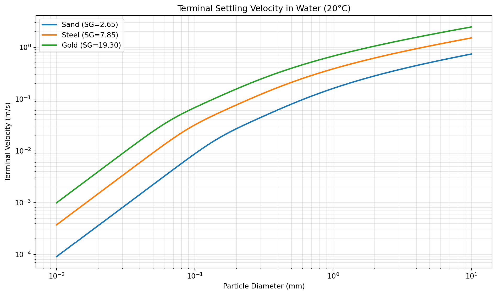
Terminal Velocity Applications. A critical application of drag calculations is determining the terminal velocity of falling particles, where the drag force balances the gravitational force. The V_TERMINAL tool solves this balance iteratively using various drag coefficient correlations. For time-dependent motion, SPHERE_VEL_AT_T calculates instantaneous velocity and SPHERE_FALL_DIST determines the distance traveled. The TIME_V_TERMINAL tool specifically calculates how long it takes a particle in the Stokes regime to approach its terminal velocity, which is important for understanding transient behavior in separators.
Choosing the Right Correlation. Selecting an appropriate correlation depends on the Reynolds number range, required accuracy, and computational efficiency. For general-purpose calculations, the DRAG_SPHERE tool automatically selects the most appropriate correlation based on the Reynolds number. For specific applications, individual correlation tools offer control over the mathematical method used. The Morsi-Alexander and Haider-Levenspiel correlations are popular for computational fluid dynamics due to their wide validity range. For educational purposes or simple Stokes-regime calculations, CD_STOKES provides the clearest physical interpretation.
Implementation. All drag calculations are implemented using NumPy for numerical operations and SciPy for iterative solution of implicit equations when calculating terminal velocity. The correlations are based on empirical fits to experimental data and theoretical analysis published in peer-reviewed fluid mechanics and chemical engineering literature.
CD_ALMEDEIJ
Computes the drag coefficient of a smooth sphere from the particle Reynolds number using the Almedeij empirical correlation. This model represents drag as a nonlinear function of Reynolds number and is intended for the published validity range.
C_D = f(Re)
Excel Usage
=CD_ALMEDEIJ(Re)Re(float, required): Particle Reynolds number [-]
Returns (float): Drag coefficient [-], or error message (str) if input is invalid.
Example 1: Reynolds number of 200
Inputs:
| Re |
|---|
| 200 |
Excel formula:
=CD_ALMEDEIJ(200)Expected output:
0.711477
Example 2: Reynolds number of 1000
Inputs:
| Re |
|---|
| 1000 |
Excel formula:
=CD_ALMEDEIJ(1000)Expected output:
0.435775
Example 3: Reynolds number of 100000
Inputs:
| Re |
|---|
| 100000 |
Excel formula:
=CD_ALMEDEIJ(100000)Expected output:
0.484339
Example 4: High Reynolds number (500000)
Inputs:
| Re |
|---|
| 500000 |
Excel formula:
=CD_ALMEDEIJ(500000)Expected output:
0.0862896
Python Code
Show Code
from fluids.drag import Almedeij as fluids_Almedeij

def cd_almedeij(Re):
    """
    Calculate drag coefficient of a sphere using the Almedeij correlation.

    See: https://fluids.readthedocs.io/fluids.drag.html#fluids.drag.Almedeij

    This example function is provided as-is without any representation of accuracy.

    Args:
        Re (float): Particle Reynolds number [-]

    Returns:
        float: Drag coefficient [-], or error message (str) if input is invalid.
    """
    try:
      Re = float(Re)
      if Re <= 0:
        return "Error: Re must be positive."

      result = fluids_Almedeij(Re=Re)
      if result != result:  # NaN check
        return "Error: Calculation resulted in NaN."
      return float(result)
    except (ValueError, TypeError):
      return "Error: Re must be a number."
    except Exception as e:
      return f"Error: {str(e)}"
Online Calculator
Particle Reynolds number [-]
CD_BARATI
Computes the drag coefficient of a smooth sphere from the particle Reynolds number using the Barati correlation. The model is an empirical fit for sphere drag over a broad intermediate Reynolds-number range.
C_D = f(Re)
Excel Usage
=CD_BARATI(Re)Re(float, required): Particle Reynolds number [-]
Returns (float): Drag coefficient [-], or error message (str) if input is invalid.
Example 1: Reynolds number of 200
Inputs:
| Re |
|---|
| 200 |
Excel formula:
=CD_BARATI(200)Expected output:
0.768224
Example 2: Reynolds number of 1000
Inputs:
| Re |
|---|
| 1000 |
Excel formula:
=CD_BARATI(1000)Expected output:
0.467423
Example 3: Reynolds number of 10000
Inputs:
| Re |
|---|
| 10000 |
Excel formula:
=CD_BARATI(10000)Expected output:
0.410781
Example 4: Reynolds number of 100000
Inputs:
| Re |
|---|
| 100000 |
Excel formula:
=CD_BARATI(100000)Expected output:
0.466713
Python Code
Show Code
from fluids.drag import Barati as fluids_Barati

def cd_barati(Re):
    """
    Calculate drag coefficient of a sphere using the Barati correlation.

    See: https://fluids.readthedocs.io/fluids.drag.html#fluids.drag.Barati

    This example function is provided as-is without any representation of accuracy.

    Args:
        Re (float): Particle Reynolds number [-]

    Returns:
        float: Drag coefficient [-], or error message (str) if input is invalid.
    """
    try:
      Re = float(Re)
      if Re <= 0:
        return "Error: Re must be positive."

      result = fluids_Barati(Re=Re)
      if result != result:  # NaN check
        return "Error: Calculation resulted in NaN."
      return float(result)
    except (ValueError, TypeError):
      return "Error: Re must be a number."
    except Exception as e:
      return f"Error: {str(e)}"
Online Calculator
Particle Reynolds number [-]
CD_BARATI_HIGH
Computes the drag coefficient of a smooth sphere from the particle Reynolds number using the high-range Barati formulation. This variant extends empirical coverage to higher Reynolds numbers than the standard Barati form.
C_D = f(Re)
Excel Usage
=CD_BARATI_HIGH(Re)Re(float, required): Particle Reynolds number [-]
Returns (float): Drag coefficient [-], or error message (str) if input is invalid.
Example 1: Reynolds number of 200
Inputs:
| Re |
|---|
| 200 |
Excel formula:
=CD_BARATI_HIGH(200)Expected output:
0.773054
Example 2: Reynolds number of 10000
Inputs:
| Re |
|---|
| 10000 |
Excel formula:
=CD_BARATI_HIGH(10000)Expected output:
0.410931
Example 3: Reynolds number of 100000
Inputs:
| Re |
|---|
| 100000 |
Excel formula:
=CD_BARATI_HIGH(100000)Expected output:
0.46701
Example 4: High Reynolds number (500000)
Inputs:
| Re |
|---|
| 500000 |
Excel formula:
=CD_BARATI_HIGH(500000)Expected output:
0.092437
Python Code
Show Code
from fluids.drag import Barati_high as fluids_Barati_high

def cd_barati_high(Re):
    """
    Calculate drag coefficient of a sphere using the Barati high-Re correlation (valid to Re=1E6).

    See: https://fluids.readthedocs.io/fluids.drag.html#fluids.drag.Barati_high

    This example function is provided as-is without any representation of accuracy.

    Args:
        Re (float): Particle Reynolds number [-]

    Returns:
        float: Drag coefficient [-], or error message (str) if input is invalid.
    """
    try:
      Re = float(Re)
      if Re <= 0:
        return "Error: Re must be positive."

      result = fluids_Barati_high(Re=Re)
      if result != result:  # NaN check
        return "Error: Calculation resulted in NaN."
      return float(result)
    except (ValueError, TypeError):
      return "Error: Re must be a number."
    except Exception as e:
      return f"Error: {str(e)}"
Online Calculator
Particle Reynolds number [-]
CD_CEYLAN
Computes the drag coefficient of a smooth sphere from the particle Reynolds number using the Ceylan correlation. The relation is an empirical expression for spherical-particle drag in external flow.
C_D = f(Re)
Excel Usage
=CD_CEYLAN(Re)Re(float, required): Particle Reynolds number [-]
Returns (float): Drag coefficient [-], or error message (str) if input is invalid.
Example 1: Reynolds number of 200
Inputs:
| Re |
|---|
| 200 |
Excel formula:
=CD_CEYLAN(200)Expected output:
0.781674
Example 2: Reynolds number of 1000
Inputs:
| Re |
|---|
| 1000 |
Excel formula:
=CD_CEYLAN(1000)Expected output:
0.523581
Example 3: Reynolds number of 100000
Inputs:
| Re |
|---|
| 100000 |
Excel formula:
=CD_CEYLAN(100000)Expected output:
0.43674
Example 4: High Reynolds number (500000)
Inputs:
| Re |
|---|
| 500000 |
Excel formula:
=CD_CEYLAN(500000)Expected output:
0.0904612
Python Code
Show Code
from fluids.drag import Ceylan as fluids_Ceylan

def cd_ceylan(Re):
    """
    Calculate drag coefficient of a sphere using the Ceylan correlation.

    See: https://fluids.readthedocs.io/fluids.drag.html#fluids.drag.Ceylan

    This example function is provided as-is without any representation of accuracy.

    Args:
        Re (float): Particle Reynolds number [-]

    Returns:
        float: Drag coefficient [-], or error message (str) if input is invalid.
    """
    try:
      Re = float(Re)
      if Re <= 0:
        return "Error: Re must be positive."

      result = fluids_Ceylan(Re=Re)
      if result != result:  # NaN check
        return "Error: Calculation resulted in NaN."
      return float(result)
    except (ValueError, TypeError):
      return "Error: Re must be a number."
    except Exception as e:
      return f"Error: {str(e)}"
Online Calculator
Particle Reynolds number [-]
CD_CHENG
Computes the drag coefficient of a smooth sphere from the particle Reynolds number using the Cheng correlation. This method blends low- and moderate-Re behavior in a compact closed-form model.
C_D = f(Re)
Excel Usage
=CD_CHENG(Re)Re(float, required): Particle Reynolds number [-]
Returns (float): Drag coefficient [-], or error message (str) if input is invalid.
Example 1: Reynolds number of 200
Inputs:
| Re |
|---|
| 200 |
Excel formula:
=CD_CHENG(200)Expected output:
0.793914
Example 2: Reynolds number of 1000
Inputs:
| Re |
|---|
| 1000 |
Excel formula:
=CD_CHENG(1000)Expected output:
0.466341
Example 3: Reynolds number of 10000
Inputs:
| Re |
|---|
| 10000 |
Excel formula:
=CD_CHENG(10000)Expected output:
0.416754
Example 4: Reynolds number of 100
Inputs:
| Re |
|---|
| 100 |
Excel formula:
=CD_CHENG(100)Expected output:
1.10238
Python Code
Show Code
from fluids.drag import Cheng as fluids_Cheng

def cd_cheng(Re):
    """
    Calculate drag coefficient of a sphere using the Cheng correlation.

    See: https://fluids.readthedocs.io/fluids.drag.html#fluids.drag.Cheng

    This example function is provided as-is without any representation of accuracy.

    Args:
        Re (float): Particle Reynolds number [-]

    Returns:
        float: Drag coefficient [-], or error message (str) if input is invalid.
    """
    try:
      Re = float(Re)
      if Re <= 0:
        return "Error: Re must be positive."

      result = fluids_Cheng(Re=Re)
      if result != result:  # NaN check
        return "Error: Calculation resulted in NaN."
      return float(result)
    except (ValueError, TypeError):
      return "Error: Re must be a number."
    except Exception as e:
      return f"Error: {str(e)}"
Online Calculator
Particle Reynolds number [-]
CD_CLIFT
Computes the drag coefficient of a smooth sphere from the particle Reynolds number using the piecewise Clift correlation. Different empirical expressions are selected across Reynolds-number intervals to capture regime-dependent drag.
C_D = f(Re)
Excel Usage
=CD_CLIFT(Re)Re(float, required): Particle Reynolds number [-]
Returns (float): Drag coefficient [-], or error message (str) if input is invalid.
Example 1: Reynolds number of 200
Inputs:
| Re |
|---|
| 200 |
Excel formula:
=CD_CLIFT(200)Expected output:
0.775634
Example 2: Reynolds number of 1000
Inputs:
| Re |
|---|
| 1000 |
Excel formula:
=CD_CLIFT(1000)Expected output:
0.471086
Example 3: Reynolds number of 100000
Inputs:
| Re |
|---|
| 100000 |
Excel formula:
=CD_CLIFT(100000)Expected output:
0.501765
Example 4: High Reynolds number (500000)
Inputs:
| Re |
|---|
| 500000 |
Excel formula:
=CD_CLIFT(500000)Expected output:
0.592804
Python Code
Show Code
from fluids.drag import Clift as fluids_Clift

def cd_clift(Re):
    """
    Calculate drag coefficient of a sphere using the Clift correlation.

    See: https://fluids.readthedocs.io/fluids.drag.html#fluids.drag.Clift

    This example function is provided as-is without any representation of accuracy.

    Args:
        Re (float): Particle Reynolds number [-]

    Returns:
        float: Drag coefficient [-], or error message (str) if input is invalid.
    """
    try:
      Re = float(Re)
      if Re <= 0:
        return "Error: Re must be positive."

      result = fluids_Clift(Re=Re)
      if result != result:  # NaN check
        return "Error: Calculation resulted in NaN."
      return float(result)
    except (ValueError, TypeError):
      return "Error: Re must be a number."
    except Exception as e:
      return f"Error: {str(e)}"
Online Calculator
Particle Reynolds number [-]
CD_CLIFT_GAUVIN
Computes the drag coefficient of a smooth sphere from the particle Reynolds number using the Clift-Gauvin correlation. The formulation combines a Stokes-like term with a high-Re correction.
C_D = f(Re)
Excel Usage
=CD_CLIFT_GAUVIN(Re)Re(float, required): Particle Reynolds number [-]
Returns (float): Drag coefficient [-], or error message (str) if input is invalid.
Example 1: Reynolds number of 200
Inputs:
| Re |
|---|
| 200 |
Excel formula:
=CD_CLIFT_GAUVIN(200)Expected output:
0.79054
Example 2: Reynolds number of 1000
Inputs:
| Re |
|---|
| 1000 |
Excel formula:
=CD_CLIFT_GAUVIN(1000)Expected output:
0.463867
Example 3: Reynolds number of 10000
Inputs:
| Re |
|---|
| 10000 |
Excel formula:
=CD_CLIFT_GAUVIN(10000)Expected output:
0.410315
Example 4: Reynolds number of 100
Inputs:
| Re |
|---|
| 100 |
Excel formula:
=CD_CLIFT_GAUVIN(100)Expected output:
1.07039
Python Code
Show Code
from fluids.drag import Clift_Gauvin as fluids_Clift_Gauvin

def cd_clift_gauvin(Re):
    """
    Calculate drag coefficient of a sphere using the Clift-Gauvin correlation.

    See: https://fluids.readthedocs.io/fluids.drag.html#fluids.drag.Clift_Gauvin

    This example function is provided as-is without any representation of accuracy.

    Args:
        Re (float): Particle Reynolds number [-]

    Returns:
        float: Drag coefficient [-], or error message (str) if input is invalid.
    """
    try:
      Re = float(Re)
      if Re <= 0:
        return "Error: Re must be positive."

      result = fluids_Clift_Gauvin(Re=Re)
      if result != result:  # NaN check
        return "Error: Calculation resulted in NaN."
      return float(result)
    except (ValueError, TypeError):
      return "Error: Re must be a number."
    except Exception as e:
      return f"Error: {str(e)}"
Online Calculator
Particle Reynolds number [-]
CD_ENGELUND
Computes the drag coefficient of a smooth sphere from the particle Reynolds number using the Engelund-Hansen correlation. The model is a simple additive form built from an inverse-Re term and a constant offset.
C_D = \frac{24}{Re} + 1.5
Excel Usage
=CD_ENGELUND(Re)Re(float, required): Particle Reynolds number [-]
Returns (float): Drag coefficient [-], or error message (str) if input is invalid.
Example 1: Reynolds number of 200
Inputs:
| Re |
|---|
| 200 |
Excel formula:
=CD_ENGELUND(200)Expected output:
1.62
Example 2: Reynolds number of 1000
Inputs:
| Re |
|---|
| 1000 |
Excel formula:
=CD_ENGELUND(1000)Expected output:
1.524
Example 3: Reynolds number of 10000
Inputs:
| Re |
|---|
| 10000 |
Excel formula:
=CD_ENGELUND(10000)Expected output:
1.5024
Example 4: Reynolds number of 100
Inputs:
| Re |
|---|
| 100 |
Excel formula:
=CD_ENGELUND(100)Expected output:
1.74
Python Code
Show Code
from fluids.drag import Engelund_Hansen as fluids_Engelund_Hansen

def cd_engelund(Re):
    """
    Calculate drag coefficient of a sphere using the Engelund-Hansen correlation.

    See: https://fluids.readthedocs.io/fluids.drag.html#fluids.drag.Engelund_Hansen

    This example function is provided as-is without any representation of accuracy.

    Args:
        Re (float): Particle Reynolds number [-]

    Returns:
        float: Drag coefficient [-], or error message (str) if input is invalid.
    """
    try:
      Re = float(Re)
      if Re <= 0:
        return "Error: Re must be positive."

      result = fluids_Engelund_Hansen(Re=Re)
      if result != result:  # NaN check
        return "Error: Calculation resulted in NaN."
      return float(result)
    except (ValueError, TypeError):
      return "Error: Re must be a number."
    except Exception as e:
      return f"Error: {str(e)}"
Online Calculator
Particle Reynolds number [-]
CD_FLEMMER_BANKS
Computes the drag coefficient of a smooth sphere from the particle Reynolds number using the Flemmer-Banks correlation. This empirical model expresses drag with a Reynolds-dependent exponent correction.
C_D = f(Re)
Excel Usage
=CD_FLEMMER_BANKS(Re)Re(float, required): Particle Reynolds number [-]
Returns (float): Drag coefficient [-], or error message (str) if input is invalid.
Example 1: Reynolds number of 200
Inputs:
| Re |
|---|
| 200 |
Excel formula:
=CD_FLEMMER_BANKS(200)Expected output:
0.784917
Example 2: Reynolds number of 1000
Inputs:
| Re |
|---|
| 1000 |
Excel formula:
=CD_FLEMMER_BANKS(1000)Expected output:
0.450582
Example 3: Reynolds number of 10000
Inputs:
| Re |
|---|
| 10000 |
Excel formula:
=CD_FLEMMER_BANKS(10000)Expected output:
0.394638
Example 4: Reynolds number of 100
Inputs:
| Re |
|---|
| 100 |
Excel formula:
=CD_FLEMMER_BANKS(100)Expected output:
1.1033
Python Code
Show Code
from fluids.drag import Flemmer_Banks as fluids_Flemmer_Banks

def cd_flemmer_banks(Re):
    """
    Calculate drag coefficient of a sphere using the Flemmer-Banks correlation.

    See: https://fluids.readthedocs.io/fluids.drag.html#fluids.drag.Flemmer_Banks

    This example function is provided as-is without any representation of accuracy.

    Args:
        Re (float): Particle Reynolds number [-]

    Returns:
        float: Drag coefficient [-], or error message (str) if input is invalid.
    """
    try:
      Re = float(Re)
      if Re <= 0:
        return "Error: Re must be positive."

      result = fluids_Flemmer_Banks(Re=Re)
      if result != result:  # NaN check
        return "Error: Calculation resulted in NaN."
      return float(result)
    except (ValueError, TypeError):
      return "Error: Re must be a number."
    except Exception as e:
      return f"Error: {str(e)}"
Online Calculator
Particle Reynolds number [-]
CD_GRAF
Computes the drag coefficient of a smooth sphere from the particle Reynolds number using the Graf correlation. The equation combines inverse-Re and transitional correction terms for spherical drag.
C_D = f(Re)
Excel Usage
=CD_GRAF(Re)Re(float, required): Particle Reynolds number [-]
Returns (float): Drag coefficient [-], or error message (str) if input is invalid.
Example 1: Reynolds number of 200
Inputs:
| Re |
|---|
| 200 |
Excel formula:
=CD_GRAF(200)Expected output:
0.852098
Example 2: Reynolds number of 1000
Inputs:
| Re |
|---|
| 1000 |
Excel formula:
=CD_GRAF(1000)Expected output:
0.49777
Example 3: Reynolds number of 10000
Inputs:
| Re |
|---|
| 10000 |
Excel formula:
=CD_GRAF(10000)Expected output:
0.324677
Example 4: Reynolds number of 100
Inputs:
| Re |
|---|
| 100 |
Excel formula:
=CD_GRAF(100)Expected output:
1.15364
Python Code
Show Code
from fluids.drag import Graf as fluids_Graf

def cd_graf(Re):
    """
    Calculate drag coefficient of a sphere using the Graf correlation.

    See: https://fluids.readthedocs.io/fluids.drag.html#fluids.drag.Graf

    This example function is provided as-is without any representation of accuracy.

    Args:
        Re (float): Particle Reynolds number [-]

    Returns:
        float: Drag coefficient [-], or error message (str) if input is invalid.
    """
    try:
      Re = float(Re)
      if Re <= 0:
        return "Error: Re must be positive."

      result = fluids_Graf(Re=Re)
      if result != result:  # NaN check
        return "Error: Calculation resulted in NaN."
      return float(result)
    except (ValueError, TypeError):
      return "Error: Re must be a number."
    except Exception as e:
      return f"Error: {str(e)}"
Online Calculator
Particle Reynolds number [-]
CD_HAIDER_LEV
Computes the drag coefficient of a smooth sphere from the particle Reynolds number using the Haider-Levenspiel correlation. The model combines a viscous-dominated term and a finite-Re correction.
C_D = f(Re)
Excel Usage
=CD_HAIDER_LEV(Re)Re(float, required): Particle Reynolds number [-]
Returns (float): Drag coefficient [-], or error message (str) if input is invalid.
Example 1: Reynolds number of 200
Inputs:
| Re |
|---|
| 200 |
Excel formula:
=CD_HAIDER_LEV(200)Expected output:
0.795955
Example 2: Reynolds number of 1000
Inputs:
| Re |
|---|
| 1000 |
Excel formula:
=CD_HAIDER_LEV(1000)Expected output:
0.453457
Example 3: Reynolds number of 10000
Inputs:
| Re |
|---|
| 10000 |
Excel formula:
=CD_HAIDER_LEV(10000)Expected output:
0.420383
Example 4: Reynolds number of 100
Inputs:
| Re |
|---|
| 100 |
Excel formula:
=CD_HAIDER_LEV(100)Expected output:
1.09474
Python Code
Show Code
from fluids.drag import Haider_Levenspiel as fluids_Haider_Levenspiel

def cd_haider_lev(Re):
    """
    Calculate drag coefficient of a sphere using the Haider-Levenspiel correlation.

    See: https://fluids.readthedocs.io/fluids.drag.html#fluids.drag.Haider_Levenspiel

    This example function is provided as-is without any representation of accuracy.

    Args:
        Re (float): Particle Reynolds number [-]

    Returns:
        float: Drag coefficient [-], or error message (str) if input is invalid.
    """
    try:
      Re = float(Re)
      if Re <= 0:
        return "Error: Re must be positive."

      result = fluids_Haider_Levenspiel(Re=Re)
      if result != result:  # NaN check
        return "Error: Calculation resulted in NaN."
      return float(result)
    except (ValueError, TypeError):
      return "Error: Re must be a number."
    except Exception as e:
      return f"Error: {str(e)}"
Online Calculator
Particle Reynolds number [-]
CD_KHAN_RICH
Computes the drag coefficient of a smooth sphere from the particle Reynolds number using the Khan-Richardson correlation. The relation is a power-law combination calibrated to spherical-particle drag data.
C_D = f(Re)
Excel Usage
=CD_KHAN_RICH(Re)Re(float, required): Particle Reynolds number [-]
Returns (float): Drag coefficient [-], or error message (str) if input is invalid.
Example 1: Reynolds number of 200
Inputs:
| Re |
|---|
| 200 |
Excel formula:
=CD_KHAN_RICH(200)Expected output:
0.774757
Example 2: Reynolds number of 1000
Inputs:
| Re |
|---|
| 1000 |
Excel formula:
=CD_KHAN_RICH(1000)Expected output:
0.48882
Example 3: Reynolds number of 10000
Inputs:
| Re |
|---|
| 10000 |
Excel formula:
=CD_KHAN_RICH(10000)Expected output:
0.403301
Example 4: Reynolds number of 100
Inputs:
| Re |
|---|
| 100 |
Excel formula:
=CD_KHAN_RICH(100)Expected output:
1.0409
Python Code
Show Code
from fluids.drag import Khan_Richardson as fluids_Khan_Richardson

def cd_khan_rich(Re):
    """
    Calculate drag coefficient of a sphere using the Khan-Richardson correlation.

    See: https://fluids.readthedocs.io/fluids.drag.html#fluids.drag.Khan_Richardson

    This example function is provided as-is without any representation of accuracy.

    Args:
        Re (float): Particle Reynolds number [-]

    Returns:
        float: Drag coefficient [-], or error message (str) if input is invalid.
    """
    try:
      Re = float(Re)
      if Re <= 0:
        return "Error: Re must be positive."

      result = fluids_Khan_Richardson(Re=Re)
      if result != result:  # NaN check
        return "Error: Calculation resulted in NaN."
      return float(result)
    except (ValueError, TypeError):
      return "Error: Re must be a number."
    except Exception as e:
      return f"Error: {str(e)}"
Online Calculator
Particle Reynolds number [-]
CD_MIKHAILOV
Computes the drag coefficient of a smooth sphere from the particle Reynolds number using the Mikhailov-Freire rational correlation. The method uses a ratio of Reynolds-number polynomials for drag estimation.
C_D = f(Re)
Excel Usage
=CD_MIKHAILOV(Re)Re(float, required): Particle Reynolds number [-]
Returns (float): Drag coefficient [-], or error message (str) if input is invalid.
Example 1: Reynolds number of 200
Inputs:
| Re |
|---|
| 200 |
Excel formula:
=CD_MIKHAILOV(200)Expected output:
0.751411
Example 2: Reynolds number of 1000
Inputs:
| Re |
|---|
| 1000 |
Excel formula:
=CD_MIKHAILOV(1000)Expected output:
0.515524
Example 3: Reynolds number of 10000
Inputs:
| Re |
|---|
| 10000 |
Excel formula:
=CD_MIKHAILOV(10000)Expected output:
0.464522
Example 4: Reynolds number of 100000
Inputs:
| Re |
|---|
| 100000 |
Excel formula:
=CD_MIKHAILOV(100000)Expected output:
0.5055
Python Code
Show Code
from fluids.drag import Mikhailov_Freire as fluids_Mikhailov_Freire

def cd_mikhailov(Re):
    """
    Calculate drag coefficient of a sphere using the Mikhailov-Freire correlation.

    See: https://fluids.readthedocs.io/fluids.drag.html#fluids.drag.Mikhailov_Freire

    This example function is provided as-is without any representation of accuracy.

    Args:
        Re (float): Particle Reynolds number [-]

    Returns:
        float: Drag coefficient [-], or error message (str) if input is invalid.
    """
    try:
      Re = float(Re)
      if Re <= 0:
        return "Error: Re must be positive."

      result = fluids_Mikhailov_Freire(Re=Re)
      if result != result:  # NaN check
        return "Error: Calculation resulted in NaN."
      return float(result)
    except (ValueError, TypeError):
      return "Error: Re must be a number."
    except Exception as e:
      return f"Error: {str(e)}"
Online Calculator
Particle Reynolds number [-]
CD_MORRISON
Computes the drag coefficient of a smooth sphere from the particle Reynolds number using the Morrison correlation. The model adds viscous, transitional, and high-Re components into one expression.
C_D = f(Re)
Excel Usage
=CD_MORRISON(Re)Re(float, required): Particle Reynolds number [-]
Returns (float): Drag coefficient [-], or error message (str) if input is invalid.
Example 1: Reynolds number of 200
Inputs:
| Re |
|---|
| 200 |
Excel formula:
=CD_MORRISON(200)Expected output:
0.767732
Example 2: Reynolds number of 1000
Inputs:
| Re |
|---|
| 1000 |
Excel formula:
=CD_MORRISON(1000)Expected output:
0.484056
Example 3: Reynolds number of 100000
Inputs:
| Re |
|---|
| 100000 |
Excel formula:
=CD_MORRISON(100000)Expected output:
0.424677
Example 4: High Reynolds number (500000)
Inputs:
| Re |
|---|
| 500000 |
Excel formula:
=CD_MORRISON(500000)Expected output:
0.0876769
Python Code
Show Code
from fluids.drag import Morrison as fluids_Morrison

def cd_morrison(Re):
    """
    Calculate drag coefficient of a sphere using the Morrison correlation.

    See: https://fluids.readthedocs.io/fluids.drag.html#fluids.drag.Morrison

    This example function is provided as-is without any representation of accuracy.

    Args:
        Re (float): Particle Reynolds number [-]

    Returns:
        float: Drag coefficient [-], or error message (str) if input is invalid.
    """
    try:
      Re = float(Re)
      if Re <= 0:
        return "Error: Re must be positive."

      result = fluids_Morrison(Re=Re)
      if result != result:  # NaN check
        return "Error: Calculation resulted in NaN."
      return float(result)
    except (ValueError, TypeError):
      return "Error: Re must be a number."
    except Exception as e:
      return f"Error: {str(e)}"
Online Calculator
Particle Reynolds number [-]
CD_MORSI_ALEX
Computes the drag coefficient of a smooth sphere from the particle Reynolds number using the Morsi-Alexander piecewise correlation. The function applies different fitted equations across Reynolds-number bands.
C_D = f(Re)
Excel Usage
=CD_MORSI_ALEX(Re)Re(float, required): Particle Reynolds number [-]
Returns (float): Drag coefficient [-], or error message (str) if input is invalid.
Example 1: Reynolds number of 200
Inputs:
| Re |
|---|
| 200 |
Excel formula:
=CD_MORSI_ALEX(200)Expected output:
0.7866
Example 2: Reynolds number of 1000
Inputs:
| Re |
|---|
| 1000 |
Excel formula:
=CD_MORSI_ALEX(1000)Expected output:
0.45812
Example 3: Reynolds number of 10000
Inputs:
| Re |
|---|
| 10000 |
Excel formula:
=CD_MORSI_ALEX(10000)Expected output:
0.407017
Example 4: Reynolds number of 100
Inputs:
| Re |
|---|
| 100 |
Excel formula:
=CD_MORSI_ALEX(100)Expected output:
1.0699
Python Code
Show Code
from fluids.drag import Morsi_Alexander as fluids_Morsi_Alexander

def cd_morsi_alex(Re):
    """
    Calculate drag coefficient of a sphere using the Morsi-Alexander correlation.

    See: https://fluids.readthedocs.io/fluids.drag.html#fluids.drag.Morsi_Alexander

    This example function is provided as-is without any representation of accuracy.

    Args:
        Re (float): Particle Reynolds number [-]

    Returns:
        float: Drag coefficient [-], or error message (str) if input is invalid.
    """
    try:
      Re = float(Re)
      if Re <= 0:
        return "Error: Re must be positive."

      result = fluids_Morsi_Alexander(Re=Re)
      if result != result:  # NaN check
        return "Error: Calculation resulted in NaN."
      return float(result)
    except (ValueError, TypeError):
      return "Error: Re must be a number."
    except Exception as e:
      return f"Error: {str(e)}"
Online Calculator
Particle Reynolds number [-]
CD_ROUSE
Computes the drag coefficient of a smooth sphere from the particle Reynolds number using the Rouse correlation. The equation combines viscous and transitional terms in a simple closed form.
C_D = \frac{24}{Re} + \frac{3}{Re^{0.5}} + 0.34
Excel Usage
=CD_ROUSE(Re)Re(float, required): Particle Reynolds number [-]
Returns (float): Drag coefficient [-], or error message (str) if input is invalid.
Example 1: Reynolds number of 200
Inputs:
| Re |
|---|
| 200 |
Excel formula:
=CD_ROUSE(200)Expected output:
0.672132
Example 2: Reynolds number of 1000
Inputs:
| Re |
|---|
| 1000 |
Excel formula:
=CD_ROUSE(1000)Expected output:
0.458868
Example 3: Reynolds number of 10000
Inputs:
| Re |
|---|
| 10000 |
Excel formula:
=CD_ROUSE(10000)Expected output:
0.3724
Example 4: Reynolds number of 100
Inputs:
| Re |
|---|
| 100 |
Excel formula:
=CD_ROUSE(100)Expected output:
0.88
Python Code
Show Code
from fluids.drag import Rouse as fluids_Rouse

def cd_rouse(Re):
    """
    Calculate drag coefficient of a sphere using the Rouse correlation.

    See: https://fluids.readthedocs.io/fluids.drag.html#fluids.drag.Rouse

    This example function is provided as-is without any representation of accuracy.

    Args:
        Re (float): Particle Reynolds number [-]

    Returns:
        float: Drag coefficient [-], or error message (str) if input is invalid.
    """
    try:
      Re = float(Re)
      if Re <= 0:
        return "Error: Re must be positive."

      result = fluids_Rouse(Re=Re)
      if result != result:  # NaN check
        return "Error: Calculation resulted in NaN."
      return float(result)
    except (ValueError, TypeError):
      return "Error: Re must be a number."
    except Exception as e:
      return f"Error: {str(e)}"
Online Calculator
Particle Reynolds number [-]
CD_SONG_XU
Computes particle drag coefficient from Reynolds number with optional shape factors using the Song-Xu correlation. The model extends beyond perfect spheres by including sphericity and projected-area ratio terms.
C_D = f(Re, \phi, S)
Excel Usage
=CD_SONG_XU(Re, sphericity, S)Re(float, required): Particle Reynolds number [-]sphericity(float, optional, default: 1): Sphericity of the particle (1.0 for sphere)S(float, optional, default: 1): Ratio of equivalent sphere area to projected area [-]
Returns (float): Drag coefficient [-], or error message (str) if input is invalid.
Example 1: Sphere at Re = 30
Inputs:
| Re |
|---|
| 30 |
Excel formula:
=CD_SONG_XU(30)Expected output:
2.34313
Example 2: Sphere at Re = 100
Inputs:
| Re |
|---|
| 100 |
Excel formula:
=CD_SONG_XU(100)Expected output:
1.16141
Example 3: Non-spherical particle
Inputs:
| Re | sphericity | S |
|---|---|---|
| 50 | 0.8 | 1.2 |
Excel formula:
=CD_SONG_XU(50, 0.8, 1.2)Expected output:
1.89685
Example 4: Cube-like particle
Inputs:
| Re | sphericity | S |
|---|---|---|
| 30 | 0.806 | 1 |
Excel formula:
=CD_SONG_XU(30, 0.806, 1)Expected output:
2.69575
Python Code
Show Code
from fluids.drag import Song_Xu as fluids_Song_Xu

def cd_song_xu(Re, sphericity=1, S=1):
    """
    Calculate drag coefficient of a particle using the Song-Xu correlation for spherical and non-spherical particles.

    See: https://fluids.readthedocs.io/fluids.drag.html#fluids.drag.Song_Xu

    This example function is provided as-is without any representation of accuracy.

    Args:
        Re (float): Particle Reynolds number [-]
        sphericity (float, optional): Sphericity of the particle (1.0 for sphere) Default is 1.
        S (float, optional): Ratio of equivalent sphere area to projected area [-] Default is 1.

    Returns:
        float: Drag coefficient [-], or error message (str) if input is invalid.
    """
    try:
      Re = float(Re)
      sphericity = float(sphericity)
      S = float(S)

      if Re <= 0:
        return "Error: Re must be positive."
      if sphericity <= 0 or sphericity > 1:
        return "Error: Sphericity must be between 0 and 1."
      if S <= 0:
        return "Error: S must be positive."

      result = fluids_Song_Xu(Re=Re, sphericity=sphericity, S=S)
      if result != result:  # NaN check
        return "Error: Calculation resulted in NaN."
      return float(result)
    except (ValueError, TypeError):
      return "Error: All parameters must be numbers."
    except Exception as e:
      return f"Error: {str(e)}"
Online Calculator
Particle Reynolds number [-]
Sphericity of the particle (1.0 for sphere)
Ratio of equivalent sphere area to projected area [-]
CD_STOKES
Computes the drag coefficient of a smooth sphere in the Stokes regime, where inertial effects are small and viscous effects dominate. The model is the classical inverse-Reynolds relation.
C_D = \frac{24}{Re}
Excel Usage
=CD_STOKES(Re)Re(float, required): Particle Reynolds number [-]
Returns (float): Drag coefficient [-], or error message (str) if input is invalid.
Example 1: Reynolds number of 0.1
Inputs:
| Re |
|---|
| 0.1 |
Excel formula:
=CD_STOKES(0.1)Expected output:
240
Example 2: Reynolds number of 0.01
Inputs:
| Re |
|---|
| 0.01 |
Excel formula:
=CD_STOKES(0.01)Expected output:
2400
Example 3: Upper validity limit (Re = 0.3)
Inputs:
| Re |
|---|
| 0.3 |
Excel formula:
=CD_STOKES(0.3)Expected output:
80
Example 4: Reynolds number of 1 (above valid range)
Inputs:
| Re |
|---|
| 1 |
Excel formula:
=CD_STOKES(1)Expected output:
24
Python Code
Show Code
from fluids.drag import Stokes as fluids_Stokes

def cd_stokes(Re):
    """
    Calculate drag coefficient of a sphere using Stokes law (Cd = 24/Re).

    See: https://fluids.readthedocs.io/fluids.drag.html#fluids.drag.Stokes

    This example function is provided as-is without any representation of accuracy.

    Args:
        Re (float): Particle Reynolds number [-]

    Returns:
        float: Drag coefficient [-], or error message (str) if input is invalid.
    """
    try:
      Re = float(Re)
      if Re <= 0:
        return "Error: Re must be positive."

      result = fluids_Stokes(Re=Re)
      if result != result:  # NaN check
        return "Error: Calculation resulted in NaN."
      return float(result)
    except (ValueError, TypeError):
      return "Error: Re must be a number."
    except Exception as e:
      return f"Error: {str(e)}"
Online Calculator
Particle Reynolds number [-]
CD_SWAMEE_OJHA
Computes the drag coefficient of a smooth sphere from the particle Reynolds number using the Swamee-Ojha correlation. The relation blends low- and high-Re behavior with a smooth empirical transition.
C_D = f(Re)
Excel Usage
=CD_SWAMEE_OJHA(Re)Re(float, required): Particle Reynolds number [-]
Returns (float): Drag coefficient [-], or error message (str) if input is invalid.
Example 1: Reynolds number of 200
Inputs:
| Re |
|---|
| 200 |
Excel formula:
=CD_SWAMEE_OJHA(200)Expected output:
0.849001
Example 2: Reynolds number of 1000
Inputs:
| Re |
|---|
| 1000 |
Excel formula:
=CD_SWAMEE_OJHA(1000)Expected output:
0.435614
Example 3: Reynolds number of 10000
Inputs:
| Re |
|---|
| 10000 |
Excel formula:
=CD_SWAMEE_OJHA(10000)Expected output:
0.420227
Example 4: Reynolds number of 100
Inputs:
| Re |
|---|
| 100 |
Excel formula:
=CD_SWAMEE_OJHA(100)Expected output:
1.18424
Python Code
Show Code
from fluids.drag import Swamee_Ojha as fluids_Swamee_Ojha

def cd_swamee_ojha(Re):
    """
    Calculate drag coefficient of a sphere using the Swamee-Ojha correlation.

    See: https://fluids.readthedocs.io/fluids.drag.html#fluids.drag.Swamee_Ojha

    This example function is provided as-is without any representation of accuracy.

    Args:
        Re (float): Particle Reynolds number [-]

    Returns:
        float: Drag coefficient [-], or error message (str) if input is invalid.
    """
    try:
      Re = float(Re)
      if Re <= 0:
        return "Error: Re must be positive."

      result = fluids_Swamee_Ojha(Re=Re)
      if result != result:  # NaN check
        return "Error: Calculation resulted in NaN."
      return float(result)
    except (ValueError, TypeError):
      return "Error: Re must be a number."
    except Exception as e:
      return f"Error: {str(e)}"
Online Calculator
Particle Reynolds number [-]
CD_TERFOUS
Computes the drag coefficient of a smooth sphere from the particle Reynolds number using the Terfous correlation. This empirical equation is calibrated for a mid-range Reynolds interval.
C_D = f(Re)
Excel Usage
=CD_TERFOUS(Re)Re(float, required): Particle Reynolds number [-]
Returns (float): Drag coefficient [-], or error message (str) if input is invalid.
Example 1: Reynolds number of 200
Inputs:
| Re |
|---|
| 200 |
Excel formula:
=CD_TERFOUS(200)Expected output:
0.781465
Example 2: Reynolds number of 1000
Inputs:
| Re |
|---|
| 1000 |
Excel formula:
=CD_TERFOUS(1000)Expected output:
0.4586
Example 3: Reynolds number of 10000
Inputs:
| Re |
|---|
| 10000 |
Excel formula:
=CD_TERFOUS(10000)Expected output:
0.400968
Example 4: Reynolds number of 100
Inputs:
| Re |
|---|
| 100 |
Excel formula:
=CD_TERFOUS(100)Expected output:
1.07088
Python Code
Show Code
from fluids.drag import Terfous as fluids_Terfous

def cd_terfous(Re):
    """
    Calculate drag coefficient of a sphere using the Terfous correlation.

    See: https://fluids.readthedocs.io/fluids.drag.html#fluids.drag.Terfous

    This example function is provided as-is without any representation of accuracy.

    Args:
        Re (float): Particle Reynolds number [-]

    Returns:
        float: Drag coefficient [-], or error message (str) if input is invalid.
    """
    try:
      Re = float(Re)
      if Re <= 0:
        return "Error: Re must be positive."

      result = fluids_Terfous(Re=Re)
      if result != result:  # NaN check
        return "Error: Calculation resulted in NaN."
      return float(result)
    except (ValueError, TypeError):
      return "Error: Re must be a number."
    except Exception as e:
      return f"Error: {str(e)}"
Online Calculator
Particle Reynolds number [-]
CD_YEN
Computes the drag coefficient of a smooth sphere from the particle Reynolds number using the Yen correlation. The formula combines a modified Stokes-like term with a corrective subtraction term.
C_D = f(Re)
Excel Usage
=CD_YEN(Re)Re(float, required): Particle Reynolds number [-]
Returns (float): Drag coefficient [-], or error message (str) if input is invalid.
Example 1: Reynolds number of 200
Inputs:
| Re |
|---|
| 200 |
Excel formula:
=CD_YEN(200)Expected output:
0.782265
Example 2: Reynolds number of 1000
Inputs:
| Re |
|---|
| 1000 |
Excel formula:
=CD_YEN(1000)Expected output:
0.545186
Example 3: Reynolds number of 10000
Inputs:
| Re |
|---|
| 10000 |
Excel formula:
=CD_YEN(10000)Expected output:
0.444341
Example 4: Reynolds number of 100
Inputs:
| Re |
|---|
| 100 |
Excel formula:
=CD_YEN(100)Expected output:
1.00779
Python Code
Show Code
from fluids.drag import Yen as fluids_Yen

def cd_yen(Re):
    """
    Calculate drag coefficient of a sphere using the Yen correlation.

    See: https://fluids.readthedocs.io/fluids.drag.html#fluids.drag.Yen

    This example function is provided as-is without any representation of accuracy.

    Args:
        Re (float): Particle Reynolds number [-]

    Returns:
        float: Drag coefficient [-], or error message (str) if input is invalid.
    """
    try:
      Re = float(Re)
      if Re <= 0:
        return "Error: Re must be positive."

      result = fluids_Yen(Re=Re)
      if result != result:  # NaN check
        return "Error: Calculation resulted in NaN."
      return float(result)
    except (ValueError, TypeError):
      return "Error: Re must be a number."
    except Exception as e:
      return f"Error: {str(e)}"
Online Calculator
Particle Reynolds number [-]
DRAG_SPHERE
Computes sphere drag coefficient by either auto-selecting a recommended correlation from Reynolds number or applying a user-specified drag model. This provides a unified interface over multiple empirical drag equations.
C_D = f(Re, \text{method})
Excel Usage
=DRAG_SPHERE(Re, drag_method)Re(float, required): Particle Reynolds number of the sphere [-]drag_method(str, optional, default: “Auto”): Correlation method to use for calculating drag coefficient
Returns (float): Drag coefficient [-], or error message (str) if input is invalid.
Example 1: Typical Reynolds number (Re = 200)
Inputs:
| Re |
|---|
| 200 |
Excel formula:
=DRAG_SPHERE(200)Expected output:
0.768224
Example 2: Low Reynolds number using Stokes region
Inputs:
| Re |
|---|
| 0.1 |
Excel formula:
=DRAG_SPHERE(0.1)Expected output:
242.658
Example 3: High Reynolds number (Re = 100000)
Inputs:
| Re |
|---|
| 100000 |
Excel formula:
=DRAG_SPHERE(100000)Expected output:
0.466713
Example 4: Using specific Rouse method
Inputs:
| Re | drag_method |
|---|---|
| 200 | Rouse |
Excel formula:
=DRAG_SPHERE(200, "Rouse")Expected output:
0.672132
Example 5: Using Morrison method
Inputs:
| Re | drag_method |
|---|---|
| 1000 | Morrison |
Excel formula:
=DRAG_SPHERE(1000, "Morrison")Expected output:
0.484056
Python Code
Show Code
from fluids.drag import drag_sphere as fluids_drag_sphere

def drag_sphere(Re, drag_method='Auto'):
    """
    Calculate the drag coefficient of a sphere using various correlations based on Reynolds number.

    See: https://fluids.readthedocs.io/fluids.drag.html#fluids.drag.drag_sphere

    This example function is provided as-is without any representation of accuracy.

    Args:
        Re (float): Particle Reynolds number of the sphere [-]
        drag_method (str, optional): Correlation method to use for calculating drag coefficient Valid options: Auto, Stokes, Barati, Barati_high, Khan_Richardson, Morsi_Alexander, Rouse, Engelund_Hansen, Clift_Gauvin, Graf, Flemmer_Banks, Swamee_Ojha, Yen, Haider_Levenspiel, Cheng, Terfous, Mikhailov_Freire, Clift, Ceylan, Almedeij, Morrison. Default is 'Auto'.

    Returns:
        float: Drag coefficient [-], or error message (str) if input is invalid.
    """
    try:
      Re = float(Re)
      if Re <= 0:
        return "Error: Re must be positive."

      # Handle method selection
      method = None if drag_method == "Auto" else drag_method

      result = fluids_drag_sphere(Re=Re, Method=method)
      if result != result:  # NaN check
        return "Error: Calculation resulted in NaN."
      return float(result)
    except (ValueError, TypeError):
      return "Error: Re must be a number."
    except Exception as e:
      return f"Error: {str(e)}"
Online Calculator
Particle Reynolds number of the sphere [-]
Correlation method to use for calculating drag coefficient
SPHERE_FALL_DIST
Computes the distance traveled by a falling sphere after a specified time by integrating the drag-governed equation of motion. It uses fluid and particle properties plus initial velocity to evolve the trajectory.
a = \frac{g(\rho_p-\rho_f)}{\rho_p} - \frac{3 C_D \rho_f u^2}{4 D \rho_p}
Excel Usage
=SPHERE_FALL_DIST(D, rhop, rho, mu, t, V)D(float, required): Diameter of the sphere [m]rhop(float, required): Particle density [kg/m^3]rho(float, required): Density of the surrounding fluid [kg/m^3]mu(float, required): Viscosity of the surrounding fluid [Pa*s]t(float, required): Time to integrate to [s]V(float, optional, default: 0): Initial velocity of the particle [m/s]
Returns (float): Distance traveled by falling sphere in time t [m], or error message (str) if invalid.
Example 1: Particle falling in air from rest
Inputs:
| D | rhop | rho | mu | t | V |
|---|---|---|---|---|---|
| 0.001 | 2200 | 1.2 | 0.0000178 | 0.5 | 0 |
Excel formula:
=SPHERE_FALL_DIST(0.001, 2200, 1.2, 0.0000178, 0.5, 0)Expected output:
1.08007
Example 2: Particle with high initial velocity
Inputs:
| D | rhop | rho | mu | t | V |
|---|---|---|---|---|---|
| 0.001 | 2200 | 1.2 | 0.0000178 | 0.5 | 30 |
Excel formula:
=SPHERE_FALL_DIST(0.001, 2200, 1.2, 0.0000178, 0.5, 30)Expected output:
7.82945
Example 3: Short integration time
Inputs:
| D | rhop | rho | mu | t | V |
|---|---|---|---|---|---|
| 0.001 | 2200 | 1.2 | 0.0000178 | 0.1 | 0 |
Excel formula:
=SPHERE_FALL_DIST(0.001, 2200, 1.2, 0.0000178, 0.1, 0)Expected output:
0.0483706
Example 4: Particle in water
Inputs:
| D | rhop | rho | mu | t | V |
|---|---|---|---|---|---|
| 0.0001 | 2600 | 1000 | 0.001 | 0.5 | 0 |
Excel formula:
=SPHERE_FALL_DIST(0.0001, 2600, 1000, 0.001, 0.5, 0)Expected output:
0.0040063
Python Code
Show Code
from fluids.drag import integrate_drag_sphere as fluids_integrate_drag_sphere

def sphere_fall_dist(D, rhop, rho, mu, t, V=0):
    """
    Calculate distance traveled by a falling sphere after a given time.

    See: https://fluids.readthedocs.io/fluids.drag.html#fluids.drag.integrate_drag_sphere

    This example function is provided as-is without any representation of accuracy.

    Args:
        D (float): Diameter of the sphere [m]
        rhop (float): Particle density [kg/m^3]
        rho (float): Density of the surrounding fluid [kg/m^3]
        mu (float): Viscosity of the surrounding fluid [Pa*s]
        t (float): Time to integrate to [s]
        V (float, optional): Initial velocity of the particle [m/s] Default is 0.

    Returns:
        float: Distance traveled by falling sphere in time t [m], or error message (str) if invalid.
    """
    try:
      D = float(D)
      rhop = float(rhop)
      rho = float(rho)
      mu = float(mu)
      t = float(t)
      V = float(V)

      if D <= 0:
        return "Error: Diameter must be positive."
      if rhop <= 0:
        return "Error: Particle density must be positive."
      if rho <= 0:
        return "Error: Fluid density must be positive."
      if mu <= 0:
        return "Error: Viscosity must be positive."
      if t < 0:
        return "Error: Time must be non-negative."

      result = fluids_integrate_drag_sphere(D=D, rhop=rhop, rho=rho, mu=mu, t=t, V=V, distance=True)
      # Returns tuple (velocity, distance) when distance=True
      distance_result = result[1]
      if distance_result != distance_result:  # NaN check
        return "Error: Calculation resulted in NaN."
      return float(distance_result)
    except (ValueError, TypeError):
      return "Error: All parameters must be numbers."
    except Exception as e:
      return f"Error: {str(e)}"
Online Calculator
Diameter of the sphere [m]
Particle density [kg/m^3]
Density of the surrounding fluid [kg/m^3]
Viscosity of the surrounding fluid [Pa*s]
Time to integrate to [s]
Initial velocity of the particle [m/s]
SPHERE_VEL_AT_T
Computes the velocity of a falling sphere at a specified time by numerically integrating the drag-governed particle dynamics. The calculation uses particle size, densities, viscosity, and initial velocity.
a = \frac{g(\rho_p-\rho_f)}{\rho_p} - \frac{3 C_D \rho_f u^2}{4 D \rho_p}
Excel Usage
=SPHERE_VEL_AT_T(D, rhop, rho, mu, t, V)D(float, required): Diameter of the sphere [m]rhop(float, required): Particle density [kg/m^3]rho(float, required): Density of the surrounding fluid [kg/m^3]mu(float, required): Viscosity of the surrounding fluid [Pa*s]t(float, required): Time to integrate to [s]V(float, optional, default: 0): Initial velocity of the particle [m/s]
Returns (float): Velocity of falling sphere after time t [m/s], or error message (str) if invalid.
Example 1: Particle falling in air from rest
Inputs:
| D | rhop | rho | mu | t | V |
|---|---|---|---|---|---|
| 0.001 | 2200 | 1.2 | 0.0000178 | 0.5 | 0 |
Excel formula:
=SPHERE_VEL_AT_T(0.001, 2200, 1.2, 0.0000178, 0.5, 0)Expected output:
3.93844
Example 2: Particle with initial velocity
Inputs:
| D | rhop | rho | mu | t | V |
|---|---|---|---|---|---|
| 0.001 | 2200 | 1.2 | 0.0000178 | 0.5 | 30 |
Excel formula:
=SPHERE_VEL_AT_T(0.001, 2200, 1.2, 0.0000178, 0.5, 30)Expected output:
9.68647
Example 3: Short integration time
Inputs:
| D | rhop | rho | mu | t | V |
|---|---|---|---|---|---|
| 0.001 | 2200 | 1.2 | 0.0000178 | 0.1 | 0 |
Excel formula:
=SPHERE_VEL_AT_T(0.001, 2200, 1.2, 0.0000178, 0.1, 0)Expected output:
0.958628
Example 4: Particle in water
Inputs:
| D | rhop | rho | mu | t | V |
|---|---|---|---|---|---|
| 0.0001 | 2600 | 1000 | 0.001 | 0.5 | 0 |
Excel formula:
=SPHERE_VEL_AT_T(0.0001, 2600, 1000, 0.001, 0.5, 0)Expected output:
0.00803345
Python Code
Show Code
from fluids.drag import integrate_drag_sphere as fluids_integrate_drag_sphere

def sphere_vel_at_t(D, rhop, rho, mu, t, V=0):
    """
    Calculate the velocity of a falling sphere after a given time.

    See: https://fluids.readthedocs.io/fluids.drag.html#fluids.drag.integrate_drag_sphere

    This example function is provided as-is without any representation of accuracy.

    Args:
        D (float): Diameter of the sphere [m]
        rhop (float): Particle density [kg/m^3]
        rho (float): Density of the surrounding fluid [kg/m^3]
        mu (float): Viscosity of the surrounding fluid [Pa*s]
        t (float): Time to integrate to [s]
        V (float, optional): Initial velocity of the particle [m/s] Default is 0.

    Returns:
        float: Velocity of falling sphere after time t [m/s], or error message (str) if invalid.
    """
    try:
      D = float(D)
      rhop = float(rhop)
      rho = float(rho)
      mu = float(mu)
      t = float(t)
      V = float(V)

      if D <= 0:
        return "Error: Diameter must be positive."
      if rhop <= 0:
        return "Error: Particle density must be positive."
      if rho <= 0:
        return "Error: Fluid density must be positive."
      if mu <= 0:
        return "Error: Viscosity must be positive."
      if t < 0:
        return "Error: Time must be non-negative."

      result = fluids_integrate_drag_sphere(D=D, rhop=rhop, rho=rho, mu=mu, t=t, V=V, distance=False)
      if result != result:  # NaN check
        return "Error: Calculation resulted in NaN."
      return float(result)
    except (ValueError, TypeError):
      return "Error: All parameters must be numbers."
    except Exception as e:
      return f"Error: {str(e)}"
Online Calculator
Diameter of the sphere [m]
Particle density [kg/m^3]
Density of the surrounding fluid [kg/m^3]
Viscosity of the surrounding fluid [Pa*s]
Time to integrate to [s]
Initial velocity of the particle [m/s]
TIME_V_TERMINAL
Computes the approximate time for a particle in the Stokes regime to approach terminal velocity from an initial velocity. Because exact convergence is asymptotic, the calculation targets a practical tolerance near terminal speed.
t_{term} \approx f(D, \rho_p, \rho_f, \mu, V_0)
Excel Usage
=TIME_V_TERMINAL(D, rhop, rho, mu, V_zero)D(float, required): Diameter of the sphere [m]rhop(float, required): Particle density [kg/m^3]rho(float, required): Density of the surrounding fluid [kg/m^3]mu(float, required): Viscosity of the surrounding fluid [Pa*s]V_zero(float, required): Initial velocity of the particle [m/s]
Returns (float): Time for particle to reach terminal velocity [s], or error message (str) if invalid.
Example 1: Tiny particle starting fast
Inputs:
| D | rhop | rho | mu | V_zero |
|---|---|---|---|---|
| 1e-7 | 2200 | 1.2 | 0.0000178 | 1 |
Excel formula:
=TIME_V_TERMINAL(1e-7, 2200, 1.2, 0.0000178, 1)Expected output:
0.000003188
Example 2: Small particle reaching terminal velocity
Inputs:
| D | rhop | rho | mu | V_zero |
|---|---|---|---|---|
| 0.00001 | 2200 | 1.2 | 0.0000178 | 0.1 |
Excel formula:
=TIME_V_TERMINAL(0.00001, 2200, 1.2, 0.0000178, 0.1)Expected output:
0.0239253
Example 3: Particle starting at rest
Inputs:
| D | rhop | rho | mu | V_zero |
|---|---|---|---|---|
| 1e-7 | 2200 | 1.2 | 0.0000178 | 0 |
Excel formula:
=TIME_V_TERMINAL(1e-7, 2200, 1.2, 0.0000178, 0)Expected output:
0.00000221382
Example 4: Particle in water
Inputs:
| D | rhop | rho | mu | V_zero |
|---|---|---|---|---|
| 0.000001 | 2600 | 1000 | 0.001 | 0.01 |
Excel formula:
=TIME_V_TERMINAL(0.000001, 2600, 1000, 0.001, 0.01)Expected output:
0.00000601411
Python Code
Show Code
from fluids.drag import time_v_terminal_Stokes as fluids_time_v_terminal_Stokes

def time_v_terminal(D, rhop, rho, mu, V_zero):
    """
    Calculate time for a particle in Stokes regime to reach terminal velocity.

    See: https://fluids.readthedocs.io/fluids.drag.html#fluids.drag.time_v_terminal_Stokes

    This example function is provided as-is without any representation of accuracy.

    Args:
        D (float): Diameter of the sphere [m]
        rhop (float): Particle density [kg/m^3]
        rho (float): Density of the surrounding fluid [kg/m^3]
        mu (float): Viscosity of the surrounding fluid [Pa*s]
        V_zero (float): Initial velocity of the particle [m/s]

    Returns:
        float: Time for particle to reach terminal velocity [s], or error message (str) if invalid.
    """
    try:
      D = float(D)
      rhop = float(rhop)
      rho = float(rho)
      mu = float(mu)
      V_zero = float(V_zero)

      if D <= 0:
        return "Error: Diameter must be positive."
      if rhop <= 0:
        return "Error: Particle density must be positive."
      if rho <= 0:
        return "Error: Fluid density must be positive."
      if mu <= 0:
        return "Error: Viscosity must be positive."

      result = fluids_time_v_terminal_Stokes(D=D, rhop=rhop, rho=rho, mu=mu, V0=V_zero)
      if result != result:  # NaN check
        return "Error: Calculation resulted in NaN."
      return float(result)
    except (ValueError, TypeError):
      return "Error: All parameters must be numbers."
    except Exception as e:
      return f"Error: {str(e)}"
Online Calculator
Diameter of the sphere [m]
Particle density [kg/m^3]
Density of the surrounding fluid [kg/m^3]
Viscosity of the surrounding fluid [Pa*s]
Initial velocity of the particle [m/s]
V_TERMINAL
Computes the terminal settling velocity of a sphere in a fluid using drag-coefficient correlations. The method solves for the velocity where net acceleration is zero under gravity, buoyancy, and drag.
v_t = \sqrt{\frac{4 g D(\rho_p-\rho_f)}{3 C_D \rho_f}}
Excel Usage
=V_TERMINAL(D, rhop, rho, mu, vt_method)D(float, required): Diameter of the sphere [m]rhop(float, required): Particle density [kg/m^3]rho(float, required): Density of the surrounding fluid [kg/m^3]mu(float, required): Viscosity of the surrounding fluid [Pa*s]vt_method(str, optional, default: “Auto”): Drag coefficient method to use
Returns (float): Terminal velocity of falling sphere [m/s], or error message (str) if input is invalid.
Example 1: Small particle (70 micron) falling in water
Inputs:
| D | rhop | rho | mu |
|---|---|---|---|
| 0.00007 | 2600 | 1000 | 0.001 |
Excel formula:
=V_TERMINAL(0.00007, 2600, 1000, 0.001)Expected output:
0.0041425
Example 2: Sand particle falling in air
Inputs:
| D | rhop | rho | mu |
|---|---|---|---|
| 0.0001 | 2500 | 1.2 | 0.0000178 |
Excel formula:
=V_TERMINAL(0.0001, 2500, 1.2, 0.0000178)Expected output:
0.555673
Example 3: Larger particle in water
Inputs:
| D | rhop | rho | mu |
|---|---|---|---|
| 0.001 | 2200 | 1000 | 0.001 |
Excel formula:
=V_TERMINAL(0.001, 2200, 1000, 0.001)Expected output:
0.128897
Example 4: Using Morrison method
Inputs:
| D | rhop | rho | mu | vt_method |
|---|---|---|---|---|
| 0.0001 | 2500 | 1.2 | 0.0000178 | Morrison |
Excel formula:
=V_TERMINAL(0.0001, 2500, 1.2, 0.0000178, "Morrison")Expected output:
0.612845
Python Code
Show Code
from fluids.drag import v_terminal as fluids_v_terminal

def v_terminal(D, rhop, rho, mu, vt_method='Auto'):
    """
    Calculate terminal velocity of a falling sphere using drag coefficient correlations.

    See: https://fluids.readthedocs.io/fluids.drag.html#fluids.drag.v_terminal

    This example function is provided as-is without any representation of accuracy.

    Args:
        D (float): Diameter of the sphere [m]
        rhop (float): Particle density [kg/m^3]
        rho (float): Density of the surrounding fluid [kg/m^3]
        mu (float): Viscosity of the surrounding fluid [Pa*s]
        vt_method (str, optional): Drag coefficient method to use Valid options: Auto, Stokes, Barati, Morrison. Default is 'Auto'.

    Returns:
        float: Terminal velocity of falling sphere [m/s], or error message (str) if input is invalid.
    """
    try:
      D = float(D)
      rhop = float(rhop)
      rho = float(rho)
      mu = float(mu)

      if D <= 0:
        return "Error: Diameter must be positive."
      if rhop <= 0:
        return "Error: Particle density must be positive."
      if rho <= 0:
        return "Error: Fluid density must be positive."
      if mu <= 0:
        return "Error: Viscosity must be positive."

      # Handle method selection
      method = None if vt_method == "Auto" else vt_method

      result = fluids_v_terminal(D=D, rhop=rhop, rho=rho, mu=mu, Method=method)
      if result != result:  # NaN check
        return "Error: Calculation resulted in NaN."
      return float(result)
    except (ValueError, TypeError):
      return "Error: All parameters must be numbers."
    except Exception as e:
      return f"Error: {str(e)}"
Online Calculator
Diameter of the sphere [m]
Particle density [kg/m^3]
Density of the surrounding fluid [kg/m^3]
Viscosity of the surrounding fluid [Pa*s]
Drag coefficient method to use