Dimensionless
Overview
Dimensionless numbers are fundamental tools in fluid mechanics and engineering that characterize the relative importance of different physical forces and phenomena. By combining variables such as velocity, length scale, fluid properties, and forces into ratios, dimensionless numbers eliminate units and reveal the underlying physics governing fluid behavior. This enables engineers to compare vastly different systems, scale experimental results, predict flow regimes, and simplify complex partial differential equations into universal forms.
The power of dimensionless analysis lies in the Buckingham π theorem, which demonstrates that any physical relationship can be expressed in terms of dimensionless groups. This foundation enables dimensional analysis, scaling laws, and similarity theory—cornerstones of experimental fluid mechanics, process design, and computational validation.
Implementation: These tools leverage the fluids Python library, which provides validated implementations of dimensionless number calculations across fluid mechanics, heat transfer, and multiphase flow. Each tool wraps a fluids.core function with consistent parameter interfaces and automatic unit handling.
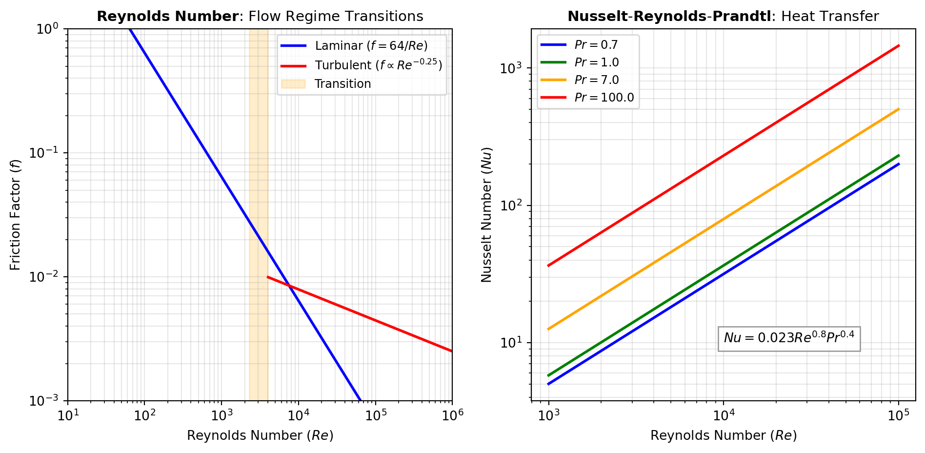
Flow Regime Numbers: Several dimensionless numbers classify flow behavior and predict regime transitions. The REYNOLDS number (Re = \rho V L / \mu) distinguishes laminar from turbulent flow, with critical values around 2300 for pipe flow. The FROUDE number (Fr = V / \sqrt{g L}) compares inertial to gravitational forces, critical for free-surface flows like open channels and ship hydrodynamics. The MACH number (Ma = V / c) compares flow velocity to sound speed, delineating subsonic, transonic, and supersonic regimes. Use these numbers to predict whether viscous, gravitational, or compressibility effects dominate.
Pressure and Force Ratios: The EULER number (Eu = \Delta p / (\rho V^2)) quantifies pressure drop relative to dynamic pressure, essential for pump and valve design. The DRAG coefficient (C_D) normalizes drag force, enabling comparison across different geometries and Reynolds numbers. The CAVITATION number (Ca = (p - p_v) / (0.5 \rho V^2)) assesses the risk of vapor bubble formation in low-pressure regions.
Surface Tension and Interfacial Flows: When surface tension dominates, the WEBER number (We = \rho V^2 L / \sigma) compares inertial to surface tension forces, critical for droplet breakup, atomization, and coating flows. The CAPILLARY number (Ca = \mu V / \sigma) balances viscous to surface tension forces, governing bubble dynamics and microfluidics. The BOND number (Bo = (\rho_L - \rho_G) g L^2 / \sigma) compares gravitational to surface tension forces, determining bubble shape and pool boiling regimes.
Heat Transfer Numbers: The NUSSELT number (Nu = h L / k) represents the ratio of convective to conductive heat transfer. Correlations typically express Nu as functions of REYNOLDS and PRANDTL numbers (Pr = \mu c_p / k), enabling prediction of heat transfer coefficients from flow conditions. The PECLET_HEAT number (Pe = Re \cdot Pr) characterizes the relative importance of advection to diffusion. For transient heat transfer, the FOURIER_HEAT number (Fo = \alpha t / L^2) measures thermal penetration depth.
Mass Transfer Numbers: Analogous to heat transfer, the SHERWOOD number (Sh = k_c L / D_{AB}) quantifies convective to diffusive mass transfer. The SCHMIDT number (Sc = \mu / (\rho D_{AB})) is the mass-transfer analog of the Prandtl number. The PECLET_MASS number (Pe = Re \cdot Sc) compares advection to diffusion, while FOURIER_MASS governs transient diffusion.
Multiphase and Buoyancy-Driven Flows: The GRASHOF number (Gr = g \beta \Delta T L^3 / \nu^2) drives natural convection, comparing buoyancy to viscous forces. The RAYLEIGH number (Ra = Gr \cdot Pr) determines convection onset in heated cavities. For particle-laden flows, the ARCHIMEDES number (Ar = g L^3 \rho_f (\rho_p - \rho_f) / \mu^2) characterizes particle settling. The CONFINEMENT number governs two-phase flow patterns in microchannels. Figure 1 illustrates how Reynolds and Froude numbers delineate flow regimes.
Common Dimensionless Groups in Engineering
Dimensionless numbers are grouped by the physical forces they balance. Understanding these ratios helps identify dominant flow features.
| Force Ratio | Dimensionless Number | Application |
|---|---|---|
| Inertial / Viscous | REYNOLDS (Re) | Turbulence, pipe flow, boundary layers |
| Inertial / Gravity | FROUDE (Fr) | Ship hulls, open channels, wave resistance |
| Inertial / Surface Tension | WEBER (We) | Droplets, bubbles, atomization |
| Viscous / Surface Tension | CAPILLARY (Ca) | Microfluidics, porous media, coating |
| Buoyancy / Viscous | GRASHOF (Gr) | Natural convection, plumes |
Python Example: Flow Classification
Using the fluids library, you can compute these numbers directly to analyze flow regimes or system stability.
from fluids.core import Froude, Capillary

# 1. Surface flow analysis (Froude)
V_ship = 15.0  # Velocity (m/s)
L_ship = 100.0 # Length (m)
g = 9.81       # Gravity (m/s^2)

Fr = Froude(V=V_ship, L=L_ship, g=g)
# Fr > 1 is supercritical; Fr < 1 is subcritical
print(f"Ship Froude Number: {Fr:.3f}")

# 2. Microfluidic channel behavior (Capillary)
V_flow = 0.05   # Velocity (m/s)
mu_oil = 0.02   # Dynamic viscosity (Pa·s)
sigma = 0.03    # Surface tension (N/m)

Ca = Capillary(V=V_flow, mu=mu_oil, sigma=sigma)
# High Ca means viscous forces dominate surface tension
print(f"Microchannel Capillary Number: {Ca:.4f}")ARCHIMEDES
Calculates the Archimedes number, a dimensionless ratio comparing buoyancy-driven forces to viscous forces for a particle in a fluid.
Excel Usage
=ARCHIMEDES(L, rhof, rhop, mu, g)L(float, required): Characteristic length (m)rhof(float, required): Density of fluid (kg/m³)rhop(float, required): Density of particle (kg/m³)mu(float, required): Dynamic viscosity of fluid (Pa·s)g(float, optional, default: 9.80665): Acceleration due to gravity (m/s²)
Returns (float): Archimedes number (float), or error message string.
Example 1: Demo case 1
Inputs:
| L | rhof | rhop | mu | g |
|---|---|---|---|---|
| 0.002 | 2 | 3000 | 0.001 | 9.80665 |
Excel formula:
=ARCHIMEDES(0.002, 2, 3000, 0.001, 9.80665)Expected output:
470.405
Example 2: Demo case 2
Inputs:
| L | rhof | rhop | mu | g |
|---|---|---|---|---|
| 0.005 | 1000 | 2500 | 0.002 | 9.81 |
Excel formula:
=ARCHIMEDES(0.005, 1000, 2500, 0.002, 9.81)Expected output:
459844
Example 3: Demo case 3
Inputs:
| L | rhof | rhop | mu | g |
|---|---|---|---|---|
| 0.01 | 800 | 1200 | 0.005 | 9.8 |
Excel formula:
=ARCHIMEDES(0.01, 800, 1200, 0.005, 9.8)Expected output:
125440
Example 4: Demo case 4
Inputs:
| L | rhof | rhop | mu | g |
|---|---|---|---|---|
| 0.002 | 2 | 3000 | 0.001 | 10 |
Excel formula:
=ARCHIMEDES(0.002, 2, 3000, 0.001, 10)Expected output:
479.68
Python Code
Show Code
from fluids.core import Archimedes as fluids_archimedes

def archimedes(L, rhof, rhop, mu, g=9.80665):
    """
    Calculate the Archimedes number (Ar) for a fluid and particle.

    See: https://fluids.readthedocs.io/fluids.core.html

    This example function is provided as-is without any representation of accuracy.

    Args:
        L (float): Characteristic length (m)
        rhof (float): Density of fluid (kg/m³)
        rhop (float): Density of particle (kg/m³)
        mu (float): Dynamic viscosity of fluid (Pa·s)
        g (float, optional): Acceleration due to gravity (m/s²) Default is 9.80665.

    Returns:
        float: Archimedes number (float), or error message string.
    """
    try:
        L_ = float(L)
        rhof_ = float(rhof)
        rhop_ = float(rhop)
        mu_ = float(mu)
        g_ = float(g)
    except (TypeError, ValueError):
        return "Error: All parameters must be numeric values."

    try:
        result = fluids_archimedes(L_, rhof_, rhop_, mu_, g_)
    except Exception as e:
        return f"Error: Failed to calculate Archimedes number: {str(e)}"

    return result
Online Calculator
Characteristic length (m)
Density of fluid (kg/m³)
Density of particle (kg/m³)
Dynamic viscosity of fluid (Pa·s)
Acceleration due to gravity (m/s²)
BEJAN
Computes the Bejan number as a pressure-drop-based dimensionless group using either a characteristic length or permeability form.
Excel Usage
=BEJAN(bejan_type, dP, L_or_K, mu, alpha)bejan_type(str, required): Calculation type for Bejan number (length-based or permeability-based)dP(float, required): Pressure drop in Pascals (Pa)L_or_K(float, required): Characteristic length (m) for length-based or permeability (m²) for permeability-basedmu(float, required): Dynamic viscosity in Pa·salpha(float, required): Thermal diffusivity in m²/s
Returns (float): Bejan number (float), or error message string.
Example 1: Demo case 1
Inputs:
| bejan_type | dP | L_or_K | mu | alpha |
|---|---|---|---|---|
| length | 10000 | 1 | 0.001 | 0.000001 |
Excel formula:
=BEJAN("length", 10000, 1, 0.001, 0.000001)Expected output:
10000000000000
Example 2: Demo case 2
Inputs:
| bejan_type | dP | L_or_K | mu | alpha |
|---|---|---|---|---|
| permeability | 10000 | 1 | 0.001 | 0.000001 |
Excel formula:
=BEJAN("permeability", 10000, 1, 0.001, 0.000001)Expected output:
10000000000000
Example 3: Demo case 3
Inputs:
| bejan_type | dP | L_or_K | mu | alpha |
|---|---|---|---|---|
| length | 500 | 0.5 | 0.002 | 0.00001 |
Excel formula:
=BEJAN("length", 500, 0.5, 0.002, 0.00001)Expected output:
6250000000
Example 4: Demo case 4
Inputs:
| bejan_type | dP | L_or_K | mu | alpha |
|---|---|---|---|---|
| permeability | 2000 | 0.05 | 0.005 | 0.00002 |
Excel formula:
=BEJAN("permeability", 2000, 0.05, 0.005, 0.00002)Expected output:
1000000000
Python Code
Show Code
from fluids import core as fluids_core

def bejan(bejan_type, dP, L_or_K, mu, alpha):
    """
    Compute the Bejan number (length-based or permeability-based).

    See: https://fluids.readthedocs.io/fluids.core.html#dimensionless-numbers

    This example function is provided as-is without any representation of accuracy.

    Args:
        bejan_type (str): Calculation type for Bejan number (length-based or permeability-based) Valid options: Length, Permeability.
        dP (float): Pressure drop in Pascals (Pa)
        L_or_K (float): Characteristic length (m) for length-based or permeability (m²) for permeability-based
        mu (float): Dynamic viscosity in Pa·s
        alpha (float): Thermal diffusivity in m²/s

    Returns:
        float: Bejan number (float), or error message string.
    """
    try:
      if not isinstance(bejan_type, str):
        return "Error: bejan_type must be a string."

      bejan_type_lower = bejan_type.lower()
      if bejan_type_lower not in ["length", "permeability"]:
        return "Error: bejan_type must be 'length' or 'permeability'."

      try:
        dP_val = float(dP)
        length_or_perm = float(L_or_K)
        mu_val = float(mu)
        alpha_val = float(alpha)
      except (TypeError, ValueError):
        return "Error: dP, L_or_K, mu, and alpha must be numeric."

      if mu_val <= 0:
        return "Error: mu (dynamic viscosity) must be positive."
      if alpha_val <= 0:
        return "Error: alpha (thermal diffusivity) must be positive."

      if bejan_type_lower == "length":
        return fluids_core.Bejan_L(dP_val, length_or_perm, mu_val, alpha_val)
      return fluids_core.Bejan_p(dP_val, length_or_perm, mu_val, alpha_val)
    except Exception as e:
        return f"Error: {str(e)}"
Online Calculator
Calculation type for Bejan number (length-based or permeability-based)
Pressure drop in Pascals (Pa)
Characteristic length (m) for length-based or permeability (m²) for permeability-based
Dynamic viscosity in Pa·s
Thermal diffusivity in m²/s
BIOT
Calculates the Biot number to compare internal conductive resistance within a body to external convective resistance at its surface.
Excel Usage
=BIOT(h, L, k)h(float, required): Heat transfer coefficient [W/m^2/K]L(float, required): Characteristic length [m]k(float, required): Thermal conductivity within the object [W/m/K]
Returns (float): Biot number [-]
Example 1: Biot number with h=1000, L=1.2, k=300
Inputs:
| h | L | k |
|---|---|---|
| 1000 | 1.2 | 300 |
Excel formula:
=BIOT(1000, 1.2, 300)Expected output:
4
Example 2: Biot number with h=10000, L=0.01, k=4000
Inputs:
| h | L | k |
|---|---|---|
| 10000 | 0.01 | 4000 |
Excel formula:
=BIOT(10000, 0.01, 4000)Expected output:
0.025
Example 3: Small Biot number (internal heat transfer dominant)
Inputs:
| h | L | k |
|---|---|---|
| 100 | 0.1 | 50 |
Excel formula:
=BIOT(100, 0.1, 50)Expected output:
0.2
Example 4: Large Biot number (surface heat transfer dominant)
Inputs:
| h | L | k |
|---|---|---|
| 5000 | 0.5 | 10 |
Excel formula:
=BIOT(5000, 0.5, 10)Expected output:
250
Python Code
Show Code
from fluids.core import Biot as fluids_Biot

def biot(h, L, k):
    """
    Calculate the Biot number for heat transfer.

    See: https://fluids.readthedocs.io/fluids.core.html#fluids.core.Biot

    This example function is provided as-is without any representation of accuracy.

    Args:
        h (float): Heat transfer coefficient [W/m^2/K]
        L (float): Characteristic length [m]
        k (float): Thermal conductivity within the object [W/m/K]

    Returns:
        float: Biot number [-]
    """
    try:
        h = float(h)
        L = float(L)
        k = float(k)

        if h < 0 or L < 0 or k <= 0:
            return "Error: h and L must be non-negative, k must be positive"

        result = fluids_Biot(h, L, k)
        return float(result)
    except (TypeError, ValueError) as e:
        return f"Error: Invalid input - {str(e)}"
    except Exception as e:
        return f"Error: {str(e)}"
Online Calculator
Heat transfer coefficient [W/m^2/K]
Characteristic length [m]
Thermal conductivity within the object [W/m/K]
BOILING
Calculates the Boiling number to relate applied heat flux to two-phase mass flux and latent heat in boiling flow.
Excel Usage
=BOILING(G, q, Hvap)G(float, required): Two-phase mass flux in kg/m²/sq(float, required): Heat flux in W/m²Hvap(float, required): Heat of vaporization in J/kg
Returns (float): Boiling number (float), or error message string.
Example 1: Demo case 1
Inputs:
| G | q | Hvap |
|---|---|---|
| 300 | 3000 | 800000 |
Excel formula:
=BOILING(300, 3000, 800000)Expected output:
0.0000125
Example 2: Demo case 2
Inputs:
| G | q | Hvap |
|---|---|---|
| 500 | 3000 | 800000 |
Excel formula:
=BOILING(500, 3000, 800000)Expected output:
0.0000075
Example 3: Demo case 3
Inputs:
| G | q | Hvap |
|---|---|---|
| 300 | 6000 | 800000 |
Excel formula:
=BOILING(300, 6000, 800000)Expected output:
0.000025
Example 4: Demo case 4
Inputs:
| G | q | Hvap |
|---|---|---|
| 300 | 3000 | 400000 |
Excel formula:
=BOILING(300, 3000, 400000)Expected output:
0.000025
Python Code
Show Code
from fluids.core import Boiling as fluids_boiling

def boiling(G, q, Hvap):
    """
    Calculate the Boiling number (Bg), a dimensionless number for boiling heat transfer.

    See: https://fluids.readthedocs.io/fluids.core.html

    This example function is provided as-is without any representation of accuracy.

    Args:
        G (float): Two-phase mass flux in kg/m²/s
        q (float): Heat flux in W/m²
        Hvap (float): Heat of vaporization in J/kg

    Returns:
        float: Boiling number (float), or error message string.
    """
    try:
        G = float(G)
        q = float(q)
        Hvap = float(Hvap)
    except (TypeError, ValueError):
        return "Error: G, q, and Hvap must be numeric values."

    if G == 0:
        return "Error: G (mass flux) must be nonzero."
    if Hvap == 0:
        return "Error: Hvap (heat of vaporization) must be nonzero."

    try:
        result = fluids_boiling(G, q, Hvap)
    except Exception as e:
        return f"Error: Failed to calculate Boiling number: {str(e)}"

    return result
Online Calculator
Two-phase mass flux in kg/m²/s
Heat flux in W/m²
Heat of vaporization in J/kg
BOND
Calculates the Bond number, which compares gravitational effects to surface tension effects for a fluid interface.
Excel Usage
=BOND(rhol, rhog, sigma, L)rhol(float, required): Density of liquid (kg/m³)rhog(float, required): Density of gas (kg/m³)sigma(float, required): Surface tension (N/m)L(float, required): Characteristic length (m)
Returns (float): Bond number [-]
Example 1: Water bubble in air
Inputs:
| rhol | rhog | sigma | L |
|---|---|---|---|
| 1000 | 1.2 | 0.0728 | 0.01 |
Excel formula:
=BOND(1000, 1.2, 0.0728, 0.01)Expected output:
13.4545
Example 2: Mercury drop in water
Inputs:
| rhol | rhog | sigma | L |
|---|---|---|---|
| 13546 | 1000 | 0.485 | 0.005 |
Excel formula:
=BOND(13546, 1000, 0.485, 0.005)Expected output:
6.34197
Example 3: Small length scale (capillary dominated)
Inputs:
| rhol | rhog | sigma | L |
|---|---|---|---|
| 800 | 1 | 0.025 | 0.0001 |
Excel formula:
=BOND(800, 1, 0.025, 0.0001)Expected output:
0.00313421
Example 4: Handbook example
Inputs:
| rhol | rhog | sigma | L |
|---|---|---|---|
| 1000 | 1.2 | 0.0589 | 2 |
Excel formula:
=BOND(1000, 1.2, 0.0589, 2)Expected output:
665187
Python Code
Show Code
from fluids.core import Bond as fluids_Bond

def bond(rhol, rhog, sigma, L):
    """
    Calculate the Bond number (Bo), also known as the Eötvös number (Eo).

    See: https://fluids.readthedocs.io/fluids.core.html#fluids.core.Bond

    This example function is provided as-is without any representation of accuracy.

    Args:
        rhol (float): Density of liquid (kg/m³)
        rhog (float): Density of gas (kg/m³)
        sigma (float): Surface tension (N/m)
        L (float): Characteristic length (m)

    Returns:
        float: Bond number [-]
    """
    try:
        return float(fluids_Bond(rhol=float(rhol), rhog=float(rhog), sigma=float(sigma), L=float(L)))
    except Exception as e:
        return f"Error: {str(e)}"
Online Calculator
Density of liquid (kg/m³)
Density of gas (kg/m³)
Surface tension (N/m)
Characteristic length (m)
CAPILLARY
Calculates the Capillary number to compare viscous forces to surface tension forces for a moving fluid.
Excel Usage
=CAPILLARY(V, mu, sigma)V(float, required): Characteristic velocity in meters per second (m/s)mu(float, required): Dynamic viscosity in Pascal-seconds (Pa·s)sigma(float, required): Surface tension in Newtons per meter (N/m)
Returns (float): The Capillary number (dimensionless). str: An error message if the input is invalid.
Example 1: Demo case 1
Inputs:
| V | mu | sigma |
|---|---|---|
| 1.2 | 0.01 | 0.1 |
Excel formula:
=CAPILLARY(1.2, 0.01, 0.1)Expected output:
0.12
Example 2: Demo case 2
Inputs:
| V | mu | sigma |
|---|---|---|
| 0.5 | 0.05 | 0.2 |
Excel formula:
=CAPILLARY(0.5, 0.05, 0.2)Expected output:
0.125
Example 3: Demo case 3
Inputs:
| V | mu | sigma |
|---|---|---|
| 2 | 0.001 | 0.5 |
Excel formula:
=CAPILLARY(2, 0.001, 0.5)Expected output:
0.004
Example 4: Demo case 4
Inputs:
| V | mu | sigma |
|---|---|---|
| 0.1 | 0.2 | 0.05 |
Excel formula:
=CAPILLARY(0.1, 0.2, 0.05)Expected output:
0.4
Python Code
Show Code
from fluids.core import Capillary as fluids_capillary

def capillary(V, mu, sigma):
    """
    Calculate the Capillary number (Ca) for a fluid system using fluids.core.Capillary.

    See: https://fluids.readthedocs.io/fluids.core.html

    This example function is provided as-is without any representation of accuracy.

    Args:
        V (float): Characteristic velocity in meters per second (m/s)
        mu (float): Dynamic viscosity in Pascal-seconds (Pa·s)
        sigma (float): Surface tension in Newtons per meter (N/m)

    Returns:
        float: The Capillary number (dimensionless). str: An error message if the input is invalid.
    """
    try:
        V_ = float(V)
        mu_ = float(mu)
        sigma_ = float(sigma)
    except (TypeError, ValueError):
        return "Error: All parameters must be numeric values."

    try:
        result = fluids_capillary(V_, mu_, sigma_)
    except (ValueError, ZeroDivisionError) as e:
        return f"Error: Failed to calculate Capillary number: {str(e)}"
    except Exception as e:
        return f"Error: {str(e)}"

    return result
Online Calculator
Characteristic velocity in meters per second (m/s)
Dynamic viscosity in Pascal-seconds (Pa·s)
Surface tension in Newtons per meter (N/m)
CAVITATION
Calculates the Cavitation number to measure how close a flowing liquid is to vapor-pressure-driven cavitation conditions.
Excel Usage
=CAVITATION(P, Psat, rho, V)P(float, required): Internal pressure in Pascals (Pa)Psat(float, required): Vapor pressure in Pascals (Pa)rho(float, required): Fluid density in kilograms per cubic meter (kg/m³)V(float, required): Fluid velocity in meters per second (m/s)
Returns (float): Cavitation number (float), or error message string.
Example 1: Demo case 1
Inputs:
| P | Psat | rho | V |
|---|---|---|---|
| 200000 | 10000 | 1000 | 10 |
Excel formula:
=CAVITATION(200000, 10000, 1000, 10)Expected output:
3.8
Example 2: Demo case 2
Inputs:
| P | Psat | rho | V |
|---|---|---|---|
| 250000 | 15000 | 950 | 20 |
Excel formula:
=CAVITATION(250000, 15000, 950, 20)Expected output:
1.23684
Example 3: Demo case 3
Inputs:
| P | Psat | rho | V |
|---|---|---|---|
| 120000 | 10000 | 998 | 8 |
Excel formula:
=CAVITATION(120000, 10000, 998, 8)Expected output:
3.44439
Example 4: Demo case 4
Inputs:
| P | Psat | rho | V |
|---|---|---|---|
| 300000 | 50000 | 1020 | 15 |
Excel formula:
=CAVITATION(300000, 50000, 1020, 15)Expected output:
2.17865
Python Code
Show Code
from fluids.core import Cavitation as fluids_cavitation

def cavitation(P, Psat, rho, V):
    """
    Calculate the Cavitation number (Ca) for a flowing fluid.

    See: https://fluids.readthedocs.io/fluids.core.html#fluids.core.Cavitation

    This example function is provided as-is without any representation of accuracy.

    Args:
        P (float): Internal pressure in Pascals (Pa)
        Psat (float): Vapor pressure in Pascals (Pa)
        rho (float): Fluid density in kilograms per cubic meter (kg/m³)
        V (float): Fluid velocity in meters per second (m/s)

    Returns:
        float: Cavitation number (float), or error message string.
    """
    try:
        P = float(P)
        Psat = float(Psat)
        rho = float(rho)
        V = float(V)
    except (ValueError, TypeError):
        return "Error: All parameters must be numeric values."

    if V == 0:
        return "Error: velocity (V) must be nonzero."
    if rho == 0:
        return "Error: density (rho) must be nonzero."

    try:
        result = fluids_cavitation(P, Psat, rho, V)
    except Exception as e:
        return f"Error: {str(e)}"
    return result
Online Calculator
Internal pressure in Pascals (Pa)
Vapor pressure in Pascals (Pa)
Fluid density in kilograms per cubic meter (kg/m³)
Fluid velocity in meters per second (m/s)
CONFINEMENT
Calculates the Confinement number for two-phase flow, relating capillary and buoyancy effects relative to channel size.
Excel Usage
=CONFINEMENT(D, rhol, rhog, sigma, g)D(float, required): Channel diameter (m)rhol(float, required): Density of liquid (kg/m³)rhog(float, required): Density of gas (kg/m³)sigma(float, required): Surface tension (N/m)g(float, optional, default: 9.80665): Acceleration due to gravity (m/s²)
Returns (float): Confinement number (float), or error message string.
Example 1: Demo case 1
Inputs:
| D | rhol | rhog | sigma | g |
|---|---|---|---|---|
| 0.001 | 1077 | 76.5 | 0.00427 | 9.80665 |
Excel formula:
=CONFINEMENT(0.001, 1077, 76.5, 0.00427, 9.80665)Expected output:
0.659698
Example 2: Demo case 2
Inputs:
| D | rhol | rhog | sigma | g |
|---|---|---|---|---|
| 0.002 | 900 | 1.2 | 0.03 | 9.80665 |
Excel formula:
=CONFINEMENT(0.002, 900, 1.2, 0.03, 9.80665)Expected output:
0.922441
Example 3: Demo case 3
Inputs:
| D | rhol | rhog | sigma | g |
|---|---|---|---|---|
| 0.0005 | 1000 | 0.6 | 0.072 | 9.80665 |
Excel formula:
=CONFINEMENT(0.0005, 1000, 0.6, 0.072, 9.80665)Expected output:
5.42084
Example 4: Demo case 4
Inputs:
| D | rhol | rhog | sigma | g |
|---|---|---|---|---|
| 0.01 | 800 | 1 | 0.002 | 9.80665 |
Excel formula:
=CONFINEMENT(0.01, 800, 1, 0.002, 9.80665)Expected output:
0.0505221
Python Code
Show Code
from fluids.core import Confinement as fluids_confinement

def confinement(D, rhol, rhog, sigma, g=9.80665):
    """
    Calculate the Confinement number (Co) for two-phase flow in a channel.

    See: https://fluids.readthedocs.io/fluids.core.html

    This example function is provided as-is without any representation of accuracy.

    Args:
        D (float): Channel diameter (m)
        rhol (float): Density of liquid (kg/m³)
        rhog (float): Density of gas (kg/m³)
        sigma (float): Surface tension (N/m)
        g (float, optional): Acceleration due to gravity (m/s²) Default is 9.80665.

    Returns:
        float: Confinement number (float), or error message string.
    """
    try:
        D = float(D)
    except (ValueError, TypeError):
        return "Error: D must be a numeric value."
    try:
        rhol = float(rhol)
    except (ValueError, TypeError):
        return "Error: rhol must be a numeric value."
    try:
        rhog = float(rhog)
    except (ValueError, TypeError):
        return "Error: rhog must be a numeric value."
    try:
        sigma = float(sigma)
    except (ValueError, TypeError):
        return "Error: sigma must be a numeric value."
    try:
        g = float(g)
    except (ValueError, TypeError):
        return "Error: g must be a numeric value."

    if D <= 0:
        return "Error: D must be positive."
    if rhol <= 0:
        return "Error: rhol must be positive."
    if rhog < 0:
        return "Error: rhog must be non-negative."
    if sigma <= 0:
        return "Error: sigma must be positive."
    if g <= 0:
        return "Error: g must be positive."
    if rhol <= rhog:
        return "Error: rhol must be greater than rhog."

    try:
        result = fluids_confinement(D, rhol, rhog, sigma, g)
    except Exception as e:
        return f"Error: Failed to calculate Confinement number: {str(e)}"
    return result
Online Calculator
Channel diameter (m)
Density of liquid (kg/m³)
Density of gas (kg/m³)
Surface tension (N/m)
Acceleration due to gravity (m/s²)
DEAN
Calculates the Dean number for curved-flow systems, combining Reynolds effects with curvature geometry.
Excel Usage
=DEAN(reynolds, inner_diameter, curvature_diameter)reynolds(float, required): Reynolds number (dimensionless)inner_diameter(float, required): Inner diameter of the pipe (m)curvature_diameter(float, required): Diameter of curvature or spiral (m)
Returns (float): Dean number (float), or error message string.
Example 1: Demo case 1
Inputs:
| reynolds | inner_diameter | curvature_diameter |
|---|---|---|
| 10000 | 0.1 | 0.4 |
Excel formula:
=DEAN(10000, 0.1, 0.4)Expected output:
5000
Example 2: Demo case 2
Inputs:
| reynolds | inner_diameter | curvature_diameter |
|---|---|---|
| 20000 | 0.2 | 0.5 |
Excel formula:
=DEAN(20000, 0.2, 0.5)Expected output:
12649.1
Example 3: Demo case 3
Inputs:
| reynolds | inner_diameter | curvature_diameter |
|---|---|---|
| 5000 | 0.05 | 0.2 |
Excel formula:
=DEAN(5000, 0.05, 0.2)Expected output:
2500
Example 4: Demo case 4
Inputs:
| reynolds | inner_diameter | curvature_diameter |
|---|---|---|
| 15000 | 0.3 | 0.3 |
Excel formula:
=DEAN(15000, 0.3, 0.3)Expected output:
15000
Python Code
Show Code
from fluids.core import Dean as fluids_dean

def dean(reynolds, inner_diameter, curvature_diameter):
    """
    Calculate the Dean number (De) for flow in a curved pipe or channel.

    See: https://fluids.readthedocs.io/en/latest/fluids.core.html#fluids.core.Dean

    This example function is provided as-is without any representation of accuracy.

    Args:
        reynolds (float): Reynolds number (dimensionless)
        inner_diameter (float): Inner diameter of the pipe (m)
        curvature_diameter (float): Diameter of curvature or spiral (m)

    Returns:
        float: Dean number (float), or error message string.
    """
    try:
        Re = float(reynolds)
        Di = float(inner_diameter)
        D = float(curvature_diameter)
    except (TypeError, ValueError):
        return "Error: All parameters must be numeric values."

    if D == 0:
        return "Error: curvature_diameter cannot be zero."

    try:
        result = fluids_dean(Re, Di, D)
    except Exception as e:
        return f"Error: {str(e)}"

    return float(result)
Online Calculator
Reynolds number (dimensionless)
Inner diameter of the pipe (m)
Diameter of curvature or spiral (m)
DRAG
Calculates the drag coefficient from force, projected area, velocity, and fluid density.
Excel Usage
=DRAG(F, A, V, rho)F(float, required): Drag force in Newtons (N)A(float, required): Projected area in square meters (m²)V(float, required): Velocity in meters per second (m/s)rho(float, required): Fluid density in kilograms per cubic meter (kg/m³)
Returns (float): Drag coefficient (float), or error message string.
Example 1: Demo case 1
Inputs:
| F | A | V | rho |
|---|---|---|---|
| 1000 | 0.0001 | 5 | 2000 |
Excel formula:
=DRAG(1000, 0.0001, 5, 2000)Expected output:
400
Example 2: Demo case 2
Inputs:
| F | A | V | rho |
|---|---|---|---|
| 500 | 0.05 | 10 | 1000 |
Excel formula:
=DRAG(500, 0.05, 10, 1000)Expected output:
0.2
Example 3: Demo case 3
Inputs:
| F | A | V | rho |
|---|---|---|---|
| 250 | 0.02 | 8 | 900 |
Excel formula:
=DRAG(250, 0.02, 8, 900)Expected output:
0.434028
Example 4: Demo case 4
Inputs:
| F | A | V | rho |
|---|---|---|---|
| 120 | 0.01 | 15 | 1.2 |
Excel formula:
=DRAG(120, 0.01, 15, 1.2)Expected output:
88.8889
Python Code
Show Code
from fluids.core import Drag as fluids_drag

def drag(F, A, V, rho):
    """
    Calculate the drag coefficient (dimensionless) for an object in a fluid.

    See: https://fluids.readthedocs.io/fluids.core.html

    This example function is provided as-is without any representation of accuracy.

    Args:
        F (float): Drag force in Newtons (N)
        A (float): Projected area in square meters (m²)
        V (float): Velocity in meters per second (m/s)
        rho (float): Fluid density in kilograms per cubic meter (kg/m³)

    Returns:
        float: Drag coefficient (float), or error message string.
    """
    try:
      F_val = float(F)
      A_val = float(A)
      V_val = float(V)
      rho_val = float(rho)

      if A_val == 0:
        return "Error: area cannot be zero."
      if V_val == 0:
        return "Error: velocity cannot be zero."
      if rho_val == 0:
        return "Error: density cannot be zero."
      if A_val < 0:
        return "Error: area must be positive."
      if rho_val < 0:
        return "Error: density must be positive."

      result = fluids_drag(F_val, A_val, V_val, rho_val)
      return float(result)
    except Exception as e:
      return f"Error: {str(e)}"
Online Calculator
Drag force in Newtons (N)
Projected area in square meters (m²)
Velocity in meters per second (m/s)
Fluid density in kilograms per cubic meter (kg/m³)
ECKERT
Calculates the Eckert number, relating kinetic energy scale to thermal enthalpy difference in flow.
Excel Usage
=ECKERT(V, Cp, dT)V(float, required): Velocity (m/s)Cp(float, required): Specific heat capacity at constant pressure (J/kg/K)dT(float, required): Temperature difference (K)
Returns (float): Eckert number (float), or error message string.
Example 1: Demo case 1
Inputs:
| V | Cp | dT |
|---|---|---|
| 10 | 2000 | 25 |
Excel formula:
=ECKERT(10, 2000, 25)Expected output:
0.002
Example 2: Demo case 2
Inputs:
| V | Cp | dT |
|---|---|---|
| 20 | 2000 | 25 |
Excel formula:
=ECKERT(20, 2000, 25)Expected output:
0.008
Example 3: Demo case 3
Inputs:
| V | Cp | dT |
|---|---|---|
| 10 | 4000 | 25 |
Excel formula:
=ECKERT(10, 4000, 25)Expected output:
0.001
Example 4: Demo case 4
Inputs:
| V | Cp | dT |
|---|---|---|
| 10 | 2000 | 50 |
Excel formula:
=ECKERT(10, 2000, 50)Expected output:
0.001
Python Code
Show Code
from fluids.core import Eckert as fluids_eckert

def eckert(V, Cp, dT):
    """
    Calculate the Eckert number using fluids.core.Eckert.

    See: https://fluids.readthedocs.io/fluids.core.html#fluids.core.Eckert

    This example function is provided as-is without any representation of accuracy.

    Args:
        V (float): Velocity (m/s)
        Cp (float): Specific heat capacity at constant pressure (J/kg/K)
        dT (float): Temperature difference (K)

    Returns:
        float: Eckert number (float), or error message string.
    """
    # Convert inputs to float
    try:
        V = float(V)
        Cp = float(Cp)
        dT = float(dT)
    except Exception:
        return "Error: All parameters must be numeric values."

    # Validate inputs
    if Cp == 0 or dT == 0:
        return "Error: Cp and dT must be nonzero."

    # Call the fluids library function
    try:
        result = fluids_eckert(V=V, Cp=Cp, dT=dT)
        return result
    except Exception as e:
        return f"Error: Failed to calculate Eckert number: {str(e)}"
Online Calculator
Velocity (m/s)
Specific heat capacity at constant pressure (J/kg/K)
Temperature difference (K)
EULER
Calculates the Euler number as the ratio of pressure-drop effects to inertial effects in a flow.
Excel Usage
=EULER(dP, rho, V)dP(float, required): Pressure drop (Pa)rho(float, required): Fluid density (kg/m³)V(float, required): Characteristic velocity (m/s)
Returns (float): Euler number (float), or error message string.
Example 1: Demo case 1
Inputs:
| dP | rho | V |
|---|---|---|
| 100000 | 1000 | 4 |
Excel formula:
=EULER(100000, 1000, 4)Expected output:
6.25
Example 2: Demo case 2
Inputs:
| dP | rho | V |
|---|---|---|
| 500 | 1.2 | 10 |
Excel formula:
=EULER(500, 1.2, 10)Expected output:
4.16667
Example 3: Demo case 3
Inputs:
| dP | rho | V |
|---|---|---|
| 2000 | 850 | 2 |
Excel formula:
=EULER(2000, 850, 2)Expected output:
0.588235
Example 4: Demo case 4
Inputs:
| dP | rho | V |
|---|---|---|
| 200000 | 2000 | 5 |
Excel formula:
=EULER(200000, 2000, 5)Expected output:
4
Python Code
Show Code
from fluids.core import Euler as fluids_euler

def euler(dP, rho, V):
    """
    Calculate the Euler number (Eu) for a fluid flow.

    See: https://fluids.readthedocs.io/fluids.core.html

    This example function is provided as-is without any representation of accuracy.

    Args:
        dP (float): Pressure drop (Pa)
        rho (float): Fluid density (kg/m³)
        V (float): Characteristic velocity (m/s)

    Returns:
        float: Euler number (float), or error message string.
    """
    try:
        dP_val = float(dP)
        rho_val = float(rho)
        V_val = float(V)
    except Exception:
        return "Error: All parameters must be numeric values."
    if rho_val == 0 or V_val == 0:
        return "Error: rho and V must be nonzero."
    try:
        result = fluids_euler(dP_val, rho_val, V_val)
    except Exception as e:
        return f"Error: {str(e)}"
    return result
Online Calculator
Pressure drop (Pa)
Fluid density (kg/m³)
Characteristic velocity (m/s)
FOURIER_HEAT
Calculates the heat-transfer Fourier number, comparing thermal diffusion over time to thermal storage length scale effects.
Excel Usage
=FOURIER_HEAT(t, L, rho, Cp, k, alpha)t(float, required): Time (s)L(float, required): Characteristic length (m)rho(float, optional, default: null): Density (kg/m³)Cp(float, optional, default: null): Heat capacity (J/kg/K)k(float, optional, default: null): Thermal conductivity (W/m/K)alpha(float, optional, default: null): Thermal diffusivity (m²/s)
Returns (float): Fourier number for heat (float), or error message string.
Example 1: Demo case 1
Inputs:
| t | L | rho | Cp | k |
|---|---|---|---|---|
| 1.5 | 2 | 1000 | 4000 | 0.6 |
Excel formula:
=FOURIER_HEAT(1.5, 2, 1000, 4000, 0.6)Expected output:
5.625e-8
Example 2: Demo case 2
Inputs:
| t | L | alpha |
|---|---|---|
| 1.5 | 2 | 1e-7 |
Excel formula:
=FOURIER_HEAT(1.5, 2, 1e-7)Expected output:
3.75e-8
Example 3: Demo case 3
Inputs:
| t | L | rho | Cp | k |
|---|---|---|---|---|
| 2 | 1 | 800 | 3800 | 0.5 |
Excel formula:
=FOURIER_HEAT(2, 1, 800, 3800, 0.5)Expected output:
3.28947e-7
Example 4: Demo case 4
Inputs:
| t | L | alpha |
|---|---|---|
| 0.5 | 0.5 | 2e-7 |
Excel formula:
=FOURIER_HEAT(0.5, 0.5, 2e-7)Expected output:
4e-7
Python Code
Show Code
from fluids.core import Fourier_heat as fluids_fourier_heat

def fourier_heat(t, L, rho=None, Cp=None, k=None, alpha=None):
    """
    Calculate the Fourier number for heat transfer.

    See: https://fluids.readthedocs.io/fluids.core.html

    This example function is provided as-is without any representation of accuracy.

    Args:
        t (float): Time (s)
        L (float): Characteristic length (m)
        rho (float, optional): Density (kg/m³) Default is None.
        Cp (float, optional): Heat capacity (J/kg/K) Default is None.
        k (float, optional): Thermal conductivity (W/m/K) Default is None.
        alpha (float, optional): Thermal diffusivity (m²/s) Default is None.

    Returns:
        float: Fourier number for heat (float), or error message string.
    """
    try:
        t_val = float(t)
        L_val = float(L)
    except Exception:
        return "Error: t and L must be numeric values."
    # If alpha is provided, use it
    if alpha is not None:
        try:
            alpha_val = float(alpha)
        except Exception:
            return "Error: alpha must be a numeric value."
        try:
            result = fluids_fourier_heat(t_val, L_val, alpha=alpha_val)
        except Exception as e:
            return f"Error: Failed to calculate Fourier number for heat: {str(e)}"
        return result
    # Otherwise, need rho, Cp, k
    if None in (rho, Cp, k):
        return "Error: must provide either alpha or all of rho, Cp, and k."
    try:
        rho_val = float(rho)
        Cp_val = float(Cp)
        k_val = float(k)
    except Exception:
        return "Error: rho, Cp, and k must be numeric values."
    try:
        result = fluids_fourier_heat(t_val, L_val, rho=rho_val, Cp=Cp_val, k=k_val)
    except Exception as e:
        return f"Error: Failed to calculate Fourier number for heat: {str(e)}"
    return result
Online Calculator
Time (s)
Characteristic length (m)
Density (kg/m³)
Heat capacity (J/kg/K)
Thermal conductivity (W/m/K)
Thermal diffusivity (m²/s)
FOURIER_MASS
Calculates the mass-transfer Fourier number to quantify diffusive transport over time relative to characteristic length.
Excel Usage
=FOURIER_MASS(t, L, D)t(float, required): Time (s)L(float, required): Characteristic length (m)D(float, required): Mass diffusivity (m²/s)
Returns (float): Fourier number for mass (float), or error message string.
Example 1: Demo case 1
Inputs:
| t | L | D |
|---|---|---|
| 1.5 | 2 | 1e-9 |
Excel formula:
=FOURIER_MASS(1.5, 2, 1e-9)Expected output:
3.75e-10
Example 2: Demo case 2
Inputs:
| t | L | D |
|---|---|---|
| 0.5 | 2 | 1e-9 |
Excel formula:
=FOURIER_MASS(0.5, 2, 1e-9)Expected output:
1.25e-10
Example 3: Demo case 3
Inputs:
| t | L | D |
|---|---|---|
| 1.5 | 4 | 1e-9 |
Excel formula:
=FOURIER_MASS(1.5, 4, 1e-9)Expected output:
9.375e-11
Example 4: Demo case 4
Inputs:
| t | L | D |
|---|---|---|
| 1.5 | 2 | 2e-9 |
Excel formula:
=FOURIER_MASS(1.5, 2, 2e-9)Expected output:
7.5e-10
Python Code
Show Code
from fluids.core import Fourier_mass as fluids_fourier_mass

def fourier_mass(t, L, D):
    """
    Calculate the Fourier number for mass transfer (Fo).

    See: https://fluids.readthedocs.io/fluids.core.html

    This example function is provided as-is without any representation of accuracy.

    Args:
        t (float): Time (s)
        L (float): Characteristic length (m)
        D (float): Mass diffusivity (m²/s)

    Returns:
        float: Fourier number for mass (float), or error message string.
    """
    try:
        t_val = float(t)
        L_val = float(L)
        D_val = float(D)
    except Exception:
        return "Error: All parameters must be numeric values."
    if L_val == 0:
        return "Error: L must not be zero."
    try:
        result = fluids_fourier_mass(t_val, L_val, D_val)
    except Exception as e:
        return f"Error: {str(e)}"
    return result
Online Calculator
Time (s)
Characteristic length (m)
Mass diffusivity (m²/s)
FROUDE
Calculates the Froude number, comparing inertial effects to gravitational effects for free-surface or gravity-influenced flow.
Excel Usage
=FROUDE(V, L, g, squared)V(float, required): Characteristic velocity (m/s)L(float, required): Characteristic length (m)g(float, optional, default: 9.80665): Gravitational acceleration (m/s²)squared(bool, optional, default: false): If true, returns squared Froude number
Returns (float): Froude number (float), or error message string.
Example 1: Demo case 1
Inputs:
| V | L | g | squared |
|---|---|---|---|
| 1.83 | 2 | 9.80665 | false |
Excel formula:
=FROUDE(1.83, 2, 9.80665, FALSE)Expected output:
0.413215
Example 2: Demo case 2
Inputs:
| V | L | g | squared |
|---|---|---|---|
| 1.83 | 2 | 1.63 | false |
Excel formula:
=FROUDE(1.83, 2, 1.63, FALSE)Expected output:
1.01354
Example 3: Demo case 3
Inputs:
| V | L | g | squared |
|---|---|---|---|
| 1.83 | 2 | 9.80665 | true |
Excel formula:
=FROUDE(1.83, 2, 9.80665, TRUE)Expected output:
0.170746
Example 4: Demo case 4
Inputs:
| V | L | g | squared |
|---|---|---|---|
| 1.83 | 2 | 1.63 | true |
Excel formula:
=FROUDE(1.83, 2, 1.63, TRUE)Expected output:
1.02727
Python Code
Show Code
from fluids.core import Froude as fluids_froude

def froude(V, L, g=9.80665, squared=False):
    """
    Calculate the Froude number (Fr) for a given velocity, length, and gravity.

    See: https://fluids.readthedocs.io/fluids.core.html#fluids.core.Froude

    This example function is provided as-is without any representation of accuracy.

    Args:
        V (float): Characteristic velocity (m/s)
        L (float): Characteristic length (m)
        g (float, optional): Gravitational acceleration (m/s²) Default is 9.80665.
        squared (bool, optional): If true, returns squared Froude number Default is False.

    Returns:
        float: Froude number (float), or error message string.
    """
    try:
        V = float(V)
        L = float(L)
        g = float(g)
        squared = bool(squared)
    except Exception:
        return "Error: V, L, and g must be numeric values."
    if L <= 0 or g <= 0:
        return "Error: L and g must be positive."
    try:
        result = fluids_froude(V, L=L, g=g, squared=squared)
    except Exception as e:
        return f"Error: {str(e)}"
    return result
Online Calculator
Characteristic velocity (m/s)
Characteristic length (m)
Gravitational acceleration (m/s²)
If true, returns squared Froude number
FROUDE_DENSIMETRIC
Calculates the densimetric Froude number for two-fluid systems, incorporating density contrast in the gravity scaling.
Excel Usage
=FROUDE_DENSIMETRIC(V, L, rho_heavy, rho_light, heavy, g)V(float, required): Velocity of the specified phase [m/s]L(float, required): Characteristic length [m]rho_heavy(float, required): Density of the heavier phase [kg/m^3]rho_light(float, required): Density of the lighter phase [kg/m^3]heavy(bool, optional, default: true): Whether to use heavy phase density in numerator (default True)g(float, optional, default: 9.80665): Acceleration due to gravity [m/s^2]
Returns (float): Densimetric Froude number [-]
Example 1: Densimetric Froude with default gravity
Inputs:
| V | L | rho_heavy | rho_light |
|---|---|---|---|
| 1.83 | 2 | 1000 | 900 |
Excel formula:
=FROUDE_DENSIMETRIC(1.83, 2, 1000, 900)Expected output:
1.3067
Example 2: Higher velocity densimetric Froude
Inputs:
| V | L | rho_heavy | rho_light |
|---|---|---|---|
| 2.5 | 1.5 | 1200 | 900 |
Excel formula:
=FROUDE_DENSIMETRIC(2.5, 1.5, 1200, 900)Expected output:
1.30366
Example 3: Densimetric Froude with heavy=False
Inputs:
| V | L | rho_heavy | rho_light | heavy |
|---|---|---|---|---|
| 1.83 | 2 | 1000 | 900 | false |
Excel formula:
=FROUDE_DENSIMETRIC(1.83, 2, 1000, 900, FALSE)Expected output:
1.23964
Example 4: Densimetric Froude with custom gravity
Inputs:
| V | L | rho_heavy | rho_light | g |
|---|---|---|---|---|
| 1.83 | 2 | 1000 | 900 | 10 |
Excel formula:
=FROUDE_DENSIMETRIC(1.83, 2, 1000, 900, 10)Expected output:
1.29401
Python Code
Show Code
from fluids.core import Froude_densimetric as fluids_Froude_densimetric

def froude_densimetric(V, L, rho_heavy, rho_light, heavy=True, g=9.80665):
    """
    Calculate the densimetric Froude number.

    See: https://fluids.readthedocs.io/fluids.core.html#fluids.core.Froude_densimetric

    This example function is provided as-is without any representation of accuracy.

    Args:
        V (float): Velocity of the specified phase [m/s]
        L (float): Characteristic length [m]
        rho_heavy (float): Density of the heavier phase [kg/m^3]
        rho_light (float): Density of the lighter phase [kg/m^3]
        heavy (bool, optional): Whether to use heavy phase density in numerator (default True) Default is True.
        g (float, optional): Acceleration due to gravity [m/s^2] Default is 9.80665.

    Returns:
        float: Densimetric Froude number [-]
    """
    try:
        V = float(V)
        L = float(L)
        rho_heavy = float(rho_heavy)
        rho_light = float(rho_light)
        heavy = bool(heavy)
        g = float(g)

        if V < 0:
            return "Error: Velocity V must be non-negative"
        if L <= 0:
            return "Error: Characteristic length L must be positive"
        if rho_heavy < 0 or rho_light < 0:
            return "Error: Densities must be non-negative"
        if rho_heavy < rho_light:
            return "Error: rho_heavy must be >= rho_light"
        if g <= 0:
            return "Error: Gravity g must be positive"

        result = fluids_Froude_densimetric(V, L, rho_heavy, rho_light, heavy, g)
        return float(result)
    except (TypeError, ValueError) as e:
        return f"Error: Invalid input - {str(e)}"
    except Exception as e:
        return f"Error: {str(e)}"
Online Calculator
Velocity of the specified phase [m/s]
Characteristic length [m]
Density of the heavier phase [kg/m^3]
Density of the lighter phase [kg/m^3]
Whether to use heavy phase density in numerator (default True)
Acceleration due to gravity [m/s^2]
GRAETZ_HEAT
Calculates the Graetz number for internal heat-transfer flow, balancing axial advection with radial thermal diffusion.
Excel Usage
=GRAETZ_HEAT(V, D, x, rho, Cp, k, alpha)V(float, required): Velocity [m/s]D(float, required): Diameter [m]x(float, required): Axial distance [m]rho(float, optional, default: null): Density [kg/m^3]Cp(float, optional, default: null): Heat capacity [J/kg/K]k(float, optional, default: null): Thermal conductivity [W/m/K]alpha(float, optional, default: null): Thermal diffusivity [m^2/s]
Returns (float): Graetz number [-]
Example 1: Example with rho, Cp, k
Inputs:
| V | D | x | rho | Cp | k |
|---|---|---|---|---|---|
| 1.5 | 0.25 | 5 | 800 | 2200 | 0.6 |
Excel formula:
=GRAETZ_HEAT(1.5, 0.25, 5, 800, 2200, 0.6)Expected output:
55000
Example 2: Example with alpha
Inputs:
| V | D | x | alpha |
|---|---|---|---|
| 1.5 | 0.25 | 5 | 1e-7 |
Excel formula:
=GRAETZ_HEAT(1.5, 0.25, 5, 1e-7)Expected output:
187500
Example 3: Smaller diameter case
Inputs:
| V | D | x | rho | Cp | k |
|---|---|---|---|---|---|
| 2 | 0.1 | 3 | 1000 | 4200 | 0.6 |
Excel formula:
=GRAETZ_HEAT(2, 0.1, 3, 1000, 4200, 0.6)Expected output:
46666.7
Example 4: Longer axial distance
Inputs:
| V | D | x | alpha |
|---|---|---|---|
| 1 | 0.3 | 10 | 2e-7 |
Excel formula:
=GRAETZ_HEAT(1, 0.3, 10, 2e-7)Expected output:
45000
Python Code
Show Code
from fluids.core import Graetz_heat as fluids_Graetz_heat

def graetz_heat(V, D, x, rho=None, Cp=None, k=None, alpha=None):
    """
    Calculate the Graetz number.

    See: https://fluids.readthedocs.io/fluids.core.html#fluids.core.Graetz_heat

    This example function is provided as-is without any representation of accuracy.

    Args:
        V (float): Velocity [m/s]
        D (float): Diameter [m]
        x (float): Axial distance [m]
        rho (float, optional): Density [kg/m^3] Default is None.
        Cp (float, optional): Heat capacity [J/kg/K] Default is None.
        k (float, optional): Thermal conductivity [W/m/K] Default is None.
        alpha (float, optional): Thermal diffusivity [m^2/s] Default is None.

    Returns:
        float: Graetz number [-]
    """
    try:
        V_val = float(V)
        D_val = float(D)
        x_val = float(x)
    except Exception:
        return "Error: V, D, and x must be numeric values."

    # Validate physical meaning
    if V_val < 0:
        return "Error: Velocity must be non-negative."
    if D_val <= 0:
        return "Error: Diameter must be positive."
    if x_val <= 0:
        return "Error: Axial distance must be positive."

    # If alpha is provided, use it
    if alpha is not None:
        try:
            alpha_val = float(alpha)
        except Exception:
            return "Error: alpha must be a numeric value."
        if alpha_val <= 0:
            return "Error: Thermal diffusivity must be positive."
        try:
            result = fluids_Graetz_heat(V_val, D_val, x_val, alpha=alpha_val)
            return float(result)
        except Exception as e:
            return f"Error: Failed to calculate Graetz number: {str(e)}"

    # Otherwise, need rho, Cp, k
    if None in (rho, Cp, k):
        return "Error: must provide either alpha or all of rho, Cp, and k."
    try:
        rho_val = float(rho)
        Cp_val = float(Cp)
        k_val = float(k)
    except Exception:
        return "Error: rho, Cp, and k must be numeric values."
    if rho_val <= 0 or Cp_val <= 0 or k_val <= 0:
        return "Error: rho, Cp, and k must all be positive."
    try:
        result = fluids_Graetz_heat(V_val, D_val, x_val, rho=rho_val, Cp=Cp_val, k=k_val)
        return float(result)
    except Exception as e:
        return f"Error: Failed to calculate Graetz number: {str(e)}"
Online Calculator
Velocity [m/s]
Diameter [m]
Axial distance [m]
Density [kg/m^3]
Heat capacity [J/kg/K]
Thermal conductivity [W/m/K]
Thermal diffusivity [m^2/s]
GRASHOF
Calculates the Grashof number to compare buoyancy forces to viscous forces in natural convection problems.
Excel Usage
=GRASHOF(L, beta, T_film, T_bulk, rho, mu, nu, g)L(float, required): Characteristic length [m]beta(float, required): Volumetric thermal expansion coefficient [1/K]T_film(float, required): Temperature 1 (film temperature) [K]T_bulk(float, optional, default: 0): Temperature 2 (bulk temperature or 0) [K]rho(float, optional, default: null): Density [kg/m^3]mu(float, optional, default: null): Dynamic viscosity [Pa*s]nu(float, optional, default: null): Kinematic viscosity [m^2/s]g(float, optional, default: 9.80665): Acceleration due to gravity [m/s^2]
Returns (float): Grashof number [-]
Example 1: Example with rho and mu
Inputs:
| L | beta | T_film | rho | mu |
|---|---|---|---|---|
| 0.9144 | 0.000933 | 178.2 | 1.1613 | 0.000019 |
Excel formula:
=GRASHOF(0.9144, 0.000933, 178.2, 1.1613, 0.000019)Expected output:
4656940000
Example 2: Example with nu and temperature difference
Inputs:
| L | beta | T_film | T_bulk | nu |
|---|---|---|---|---|
| 0.9144 | 0.000933 | 378.2 | 200 | 0.00001636 |
Excel formula:
=GRASHOF(0.9144, 0.000933, 378.2, 200, 0.00001636)Expected output:
4657490000
Example 3: Larger characteristic length
Inputs:
| L | beta | T_film | rho | mu |
|---|---|---|---|---|
| 1.5 | 0.0008 | 200 | 1.2 | 0.00002 |
Excel formula:
=GRASHOF(1.5, 0.0008, 200, 1.2, 0.00002)Expected output:
19064100000
Example 4: Smaller characteristic length
Inputs:
| L | beta | T_film | nu |
|---|---|---|---|
| 0.1 | 0.001 | 150 | 0.000015 |
Excel formula:
=GRASHOF(0.1, 0.001, 150, 0.000015)Expected output:
6537770
Python Code
Show Code
from fluids.core import Grashof as fluids_Grashof

def grashof(L, beta, T_film, T_bulk=0, rho=None, mu=None, nu=None, g=9.80665):
    """
    Calculate the Grashof number.

    See: https://fluids.readthedocs.io/fluids.core.html#fluids.core.Grashof

    This example function is provided as-is without any representation of accuracy.

    Args:
        L (float): Characteristic length [m]
        beta (float): Volumetric thermal expansion coefficient [1/K]
        T_film (float): Temperature 1 (film temperature) [K]
        T_bulk (float, optional): Temperature 2 (bulk temperature or 0) [K] Default is 0.
        rho (float, optional): Density [kg/m^3] Default is None.
        mu (float, optional): Dynamic viscosity [Pa*s] Default is None.
        nu (float, optional): Kinematic viscosity [m^2/s] Default is None.
        g (float, optional): Acceleration due to gravity [m/s^2] Default is 9.80665.

    Returns:
        float: Grashof number [-]
    """
    try:
        L_val = float(L)
        beta_val = float(beta)
        T_film_val = float(T_film)
        T_bulk_val = float(T_bulk) if T_bulk is not None else 0
    except Exception:
        return "Error: L, beta, T_film, and T_bulk must be numeric values."

    # Validate physical meaning
    if L_val <= 0:
        return "Error: Characteristic length must be positive."
    if beta_val <= 0:
        return "Error: Volumetric thermal expansion coefficient must be positive."

    # Check if nu is provided
    if nu is not None:
        try:
            nu_val = float(nu)
        except Exception:
            return "Error: nu must be a numeric value."
        if nu_val <= 0:
            return "Error: Kinematic viscosity must be positive."
        try:
            g_val = float(g) if g is not None else 9.80665
            result = fluids_Grashof(L_val, beta_val, T_film_val, T_bulk_val, nu=nu_val, g=g_val)
            return float(result)
        except Exception as e:
            return f"Error: Failed to calculate Grashof number: {str(e)}"

    # Otherwise, need rho and mu
    if None in (rho, mu):
        return "Error: must provide either nu or both rho and mu."
    try:
        rho_val = float(rho)
        mu_val = float(mu)
        g_val = float(g) if g is not None else 9.80665
    except Exception:
        return "Error: rho, mu, and g must be numeric values."
    if rho_val <= 0 or mu_val <= 0:
        return "Error: rho and mu must both be positive."
    try:
        result = fluids_Grashof(L_val, beta_val, T_film_val, T_bulk_val, rho=rho_val, mu=mu_val, g=g_val)
        return float(result)
    except Exception as e:
        return f"Error: Failed to calculate Grashof number: {str(e)}"
Online Calculator
Characteristic length [m]
Volumetric thermal expansion coefficient [1/K]
Temperature 1 (film temperature) [K]
Temperature 2 (bulk temperature or 0) [K]
Density [kg/m^3]
Dynamic viscosity [Pa*s]
Kinematic viscosity [m^2/s]
Acceleration due to gravity [m/s^2]
HAGEN
Calculates the Hagen number from Reynolds number and Darcy friction factor for internal-flow correlation work.
Excel Usage
=HAGEN(Re, fd)Re(float, required): Reynolds number [-]fd(float, required): Darcy friction factor [-]
Returns (float): Hagen number [-]
Example 1: VDI example with Re=2610, fd=1.935235
Inputs:
| Re | fd |
|---|---|
| 2610 | 1.935235 |
Excel formula:
=HAGEN(2610, 1.935235)Expected output:
6591510
Example 2: Laminar flow case
Inputs:
| Re | fd |
|---|---|
| 100 | 0.64 |
Excel formula:
=HAGEN(100, 0.64)Expected output:
3200
Example 3: Turbulent flow case
Inputs:
| Re | fd |
|---|---|
| 10000 | 0.03164 |
Excel formula:
=HAGEN(10000, 0.03164)Expected output:
1582000
Example 4: High friction factor case
Inputs:
| Re | fd |
|---|---|
| 5000 | 0.5 |
Excel formula:
=HAGEN(5000, 0.5)Expected output:
6250000
Python Code
Show Code
from fluids.core import Hagen as fluids_Hagen

def hagen(Re, fd):
    """
    Calculate the Hagen number.

    See: https://fluids.readthedocs.io/fluids.core.html#fluids.core.Hagen

    This example function is provided as-is without any representation of accuracy.

    Args:
        Re (float): Reynolds number [-]
        fd (float): Darcy friction factor [-]

    Returns:
        float: Hagen number [-]
    """
    try:
        Re = float(Re)
        fd = float(fd)

        if Re < 0:
            return "Error: Reynolds number Re must be non-negative"
        if fd < 0:
            return "Error: Darcy friction factor fd must be non-negative"

        result = fluids_Hagen(Re, fd)
        return float(result)
    except (TypeError, ValueError) as e:
        return f"Error: Invalid input - {str(e)}"
    except Exception as e:
        return f"Error: {str(e)}"
Online Calculator
Reynolds number [-]
Darcy friction factor [-]
JAKOB
Calculates the Jakob number, relating sensible heat capacity effects to latent heat effects in boiling.
Excel Usage
=JAKOB(Cp, Hvap, Te)Cp(float, required): Heat capacity of the fluid [J/kg/K]Hvap(float, required): Enthalpy of vaporization [J/kg]Te(float, required): Temperature difference above saturation boiling temperature [K]
Returns (float): Jakob number [-]
Example 1: Water boiling with Cp=4000, Hvap=2E6, Te=10
Inputs:
| Cp | Hvap | Te |
|---|---|---|
| 4000 | 2000000 | 10 |
Excel formula:
=JAKOB(4000, 2000000, 10)Expected output:
0.02
Example 2: Small superheat (Jakob < 1)
Inputs:
| Cp | Hvap | Te |
|---|---|---|
| 2000 | 2500000 | 5 |
Excel formula:
=JAKOB(2000, 2500000, 5)Expected output:
0.004
Example 3: Large superheat
Inputs:
| Cp | Hvap | Te |
|---|---|---|
| 3500 | 1500000 | 30 |
Excel formula:
=JAKOB(3500, 1500000, 30)Expected output:
0.07
Example 4: Fluid with high heat capacity
Inputs:
| Cp | Hvap | Te |
|---|---|---|
| 6000 | 2000000 | 15 |
Excel formula:
=JAKOB(6000, 2000000, 15)Expected output:
0.045
Python Code
Show Code
from fluids.core import Jakob as fluids_Jakob

def jakob(Cp, Hvap, Te):
    """
    Calculate the Jakob number for boiling fluid.

    See: https://fluids.readthedocs.io/fluids.core.html#fluids.core.Jakob

    This example function is provided as-is without any representation of accuracy.

    Args:
        Cp (float): Heat capacity of the fluid [J/kg/K]
        Hvap (float): Enthalpy of vaporization [J/kg]
        Te (float): Temperature difference above saturation boiling temperature [K]

    Returns:
        float: Jakob number [-]
    """
    try:
        Cp = float(Cp)
        Hvap = float(Hvap)
        Te = float(Te)

        if Cp < 0:
            return "Error: Heat capacity Cp must be non-negative"
        if Hvap <= 0:
            return "Error: Enthalpy of vaporization Hvap must be positive"
        if Te < 0:
            return "Error: Temperature difference Te must be non-negative"

        result = fluids_Jakob(Cp, Hvap, Te)
        return float(result)
    except (TypeError, ValueError) as e:
        return f"Error: Invalid input - {str(e)}"
    except Exception as e:
        return f"Error: {str(e)}"
Online Calculator
Heat capacity of the fluid [J/kg/K]
Enthalpy of vaporization [J/kg]
Temperature difference above saturation boiling temperature [K]
KNUDSEN
Calculates the Knudsen number as the ratio of molecular mean free path to characteristic geometric length.
Excel Usage
=KNUDSEN(path, L)path(float, required): Mean free path between molecular collisions [m]L(float, required): Characteristic length [m]
Returns (float): Knudsen number [-]
Example 1: Knudsen number with path=1e-10, L=0.001
Inputs:
| path | L |
|---|---|
| 1e-10 | 0.001 |
Excel formula:
=KNUDSEN(1e-10, 0.001)Expected output:
1e-7
Example 2: Continuum flow regime (Kn << 1)
Inputs:
| path | L |
|---|---|
| 1e-8 | 0.01 |
Excel formula:
=KNUDSEN(1e-8, 0.01)Expected output:
0.000001
Example 3: Transition flow regime (Kn ~ 1)
Inputs:
| path | L |
|---|---|
| 0.00001 | 0.00001 |
Excel formula:
=KNUDSEN(0.00001, 0.00001)Expected output:
1
Example 4: Free molecular flow regime (Kn >> 1)
Inputs:
| path | L |
|---|---|
| 0.001 | 0.000001 |
Excel formula:
=KNUDSEN(0.001, 0.000001)Expected output:
1000
Python Code
Show Code
from fluids.core import Knudsen as fluids_Knudsen

def knudsen(path, L):
    """
    Calculate the Knudsen number.

    See: https://fluids.readthedocs.io/fluids.core.html#fluids.core.Knudsen

    This example function is provided as-is without any representation of accuracy.

    Args:
        path (float): Mean free path between molecular collisions [m]
        L (float): Characteristic length [m]

    Returns:
        float: Knudsen number [-]
    """
    try:
        path = float(path)
        L = float(L)

        if path < 0:
            return "Error: Mean free path must be non-negative"
        if L <= 0:
            return "Error: Characteristic length L must be positive"

        result = fluids_Knudsen(path, L)
        return float(result)
    except (TypeError, ValueError) as e:
        return f"Error: Invalid input - {str(e)}"
    except Exception as e:
        return f"Error: {str(e)}"
Online Calculator
Mean free path between molecular collisions [m]
Characteristic length [m]
LEWIS
Calculates the Lewis number to compare thermal diffusivity and mass diffusivity in coupled heat and mass transfer.
Excel Usage
=LEWIS(D, alpha, Cp, k, rho)D(float, required): Diffusivity of a species [m^2/s]alpha(float, optional, default: null): Thermal diffusivity [m^2/s]Cp(float, optional, default: null): Heat capacity [J/kg/K]k(float, optional, default: null): Thermal conductivity [W/m/K]rho(float, optional, default: null): Density [kg/m^3]
Returns (float): Lewis number [-]
Example 1: Example with alpha
Inputs:
| D | alpha |
|---|---|
| 0.0000226 | 0.0000191 |
Excel formula:
=LEWIS(0.0000226, 0.0000191)Expected output:
0.845133
Example 2: Example with rho, Cp, k
Inputs:
| D | rho | k | Cp |
|---|---|---|---|
| 0.0000226 | 800 | 0.2 | 2200 |
Excel formula:
=LEWIS(0.0000226, 800, 0.2, 2200)Expected output:
0.00502816
Example 3: Higher diffusivity with alpha
Inputs:
| D | alpha |
|---|---|
| 0.00003 | 0.00002 |
Excel formula:
=LEWIS(0.00003, 0.00002)Expected output:
0.666667
Example 4: Water with thermal properties
Inputs:
| D | rho | Cp | k |
|---|---|---|---|
| 0.000025 | 998 | 4182 | 0.6 |
Excel formula:
=LEWIS(0.000025, 998, 4182, 0.6)Expected output:
0.00575038
Python Code
Show Code
from fluids.core import Lewis as fluids_Lewis

def lewis(D, alpha=None, Cp=None, k=None, rho=None):
    """
    Calculate the Lewis number.

    See: https://fluids.readthedocs.io/fluids.core.html#fluids.core.Lewis

    This example function is provided as-is without any representation of accuracy.

    Args:
        D (float): Diffusivity of a species [m^2/s]
        alpha (float, optional): Thermal diffusivity [m^2/s] Default is None.
        Cp (float, optional): Heat capacity [J/kg/K] Default is None.
        k (float, optional): Thermal conductivity [W/m/K] Default is None.
        rho (float, optional): Density [kg/m^3] Default is None.

    Returns:
        float: Lewis number [-]
    """
    try:
        D_val = float(D)
    except Exception:
        return "Error: D must be a numeric value."

    # Validate physical meaning
    if D_val <= 0:
        return "Error: Diffusivity must be positive."

    # If alpha is provided, use it
    if alpha is not None:
        try:
            alpha_val = float(alpha)
        except Exception:
            return "Error: alpha must be a numeric value."
        if alpha_val <= 0:
            return "Error: Thermal diffusivity must be positive."
        try:
            result = fluids_Lewis(D_val, alpha=alpha_val)
            return float(result)
        except Exception as e:
            return f"Error: Failed to calculate Lewis number: {str(e)}"

    # Otherwise, need rho, Cp, k
    if None in (Cp, k, rho):
        return "Error: must provide either alpha or all of rho, Cp, and k."
    try:
        Cp_val = float(Cp)
        k_val = float(k)
        rho_val = float(rho)
    except Exception:
        return "Error: Cp, k, and rho must be numeric values."
    if rho_val <= 0 or Cp_val <= 0 or k_val <= 0:
        return "Error: rho, Cp, and k must all be positive."
    try:
        result = fluids_Lewis(D_val, Cp=Cp_val, k=k_val, rho=rho_val)
        return float(result)
    except Exception as e:
        return f"Error: Failed to calculate Lewis number: {str(e)}"
Online Calculator
Diffusivity of a species [m^2/s]
Thermal diffusivity [m^2/s]
Heat capacity [J/kg/K]
Thermal conductivity [W/m/K]
Density [kg/m^3]
MACH
Calculates the Mach number as the ratio of fluid velocity to local speed of sound.
Excel Usage
=MACH(V, c)V(float, required): Velocity of fluid [m/s]c(float, required): Speed of sound in fluid [m/s]
Returns (float): Mach number [-]
Example 1: Subsonic flow (Mach < 1)
Inputs:
| V | c |
|---|---|
| 33 | 330 |
Excel formula:
=MACH(33, 330)Expected output:
0.1
Example 2: Sonic flow (Mach = 1)
Inputs:
| V | c |
|---|---|
| 340 | 340 |
Excel formula:
=MACH(340, 340)Expected output:
1
Example 3: Supersonic flow (Mach > 1)
Inputs:
| V | c |
|---|---|
| 500 | 340 |
Excel formula:
=MACH(500, 340)Expected output:
1.47059
Example 4: Low velocity example
Inputs:
| V | c |
|---|---|
| 10 | 300 |
Excel formula:
=MACH(10, 300)Expected output:
0.0333333
Python Code
Show Code
from fluids.core import Mach as fluids_Mach

def mach(V, c):
    """
    Calculate the Mach number.

    See: https://fluids.readthedocs.io/fluids.core.html#fluids.core.Mach

    This example function is provided as-is without any representation of accuracy.

    Args:
        V (float): Velocity of fluid [m/s]
        c (float): Speed of sound in fluid [m/s]

    Returns:
        float: Mach number [-]
    """
    try:
      V_val = float(V)
      c_val = float(c)

      if c_val <= 0:
        return "Error: Speed of sound must be positive"

      result = fluids_Mach(V_val, c_val)
      return float(result)
    except Exception as e:
      return f"Error: {str(e)}"
Online Calculator
Velocity of fluid [m/s]
Speed of sound in fluid [m/s]
MORTON
Calculates the Morton number for gas-liquid systems to characterize fluid-property control of bubble behavior.
Excel Usage
=MORTON(rhol, rhog, mul, sigma, g)rhol(float, required): Density of liquid phase [kg/m^3]rhog(float, required): Density of gas phase [kg/m^3]mul(float, required): Viscosity of liquid phase [Pa*s]sigma(float, required): Surface tension between liquid-gas phase [N/m]g(float, optional, default: 9.80665): Acceleration due to gravity [m/s^2]
Returns (float): Morton number [-]
Example 1: Water-air system
Inputs:
| rhol | rhog | mul | sigma |
|---|---|---|---|
| 1077 | 76.5 | 0.00427 | 0.023 |
Excel formula:
=MORTON(1077, 76.5, 0.00427, 0.023)Expected output:
2.31118e-7
Example 2: High surface tension case
Inputs:
| rhol | rhog | mul | sigma |
|---|---|---|---|
| 1000 | 1 | 0.001 | 0.1 |
Excel formula:
=MORTON(1000, 1, 0.001, 0.1)Expected output:
9.79684e-12
Example 3: Low viscosity liquid
Inputs:
| rhol | rhog | mul | sigma |
|---|---|---|---|
| 800 | 2 | 0.0001 | 0.03 |
Excel formula:
=MORTON(800, 2, 0.0001, 0.03)Expected output:
4.52877e-14
Example 4: Custom gravity value
Inputs:
| rhol | rhog | mul | sigma | g |
|---|---|---|---|---|
| 1000 | 10 | 0.002 | 0.05 | 3.71 |
Excel formula:
=MORTON(1000, 10, 0.002, 0.05, 3.71)Expected output:
4.70131e-10
Python Code
Show Code
from fluids.core import Morton as fluids_Morton

def morton(rhol, rhog, mul, sigma, g=9.80665):
    """
    Calculate the Morton number.

    See: https://fluids.readthedocs.io/fluids.core.html#fluids.core.Morton

    This example function is provided as-is without any representation of accuracy.

    Args:
        rhol (float): Density of liquid phase [kg/m^3]
        rhog (float): Density of gas phase [kg/m^3]
        mul (float): Viscosity of liquid phase [Pa*s]
        sigma (float): Surface tension between liquid-gas phase [N/m]
        g (float, optional): Acceleration due to gravity [m/s^2] Default is 9.80665.

    Returns:
        float: Morton number [-]
    """
    try:
      rhol_val = float(rhol)
      rhog_val = float(rhog)
      mul_val = float(mul)
      sigma_val = float(sigma)
      g_val = float(g)

      if rhol_val <= 0 or mul_val <= 0 or sigma_val <= 0 or g_val <= 0:
        return "Error: Density, viscosity, surface tension, and gravity must be positive"

      result = fluids_Morton(rhol_val, rhog_val, mul_val, sigma_val, g_val)
      return float(result)
    except Exception as e:
      return f"Error: {str(e)}"
Online Calculator
Density of liquid phase [kg/m^3]
Density of gas phase [kg/m^3]
Viscosity of liquid phase [Pa*s]
Surface tension between liquid-gas phase [N/m]
Acceleration due to gravity [m/s^2]
NUSSELT
Calculates the Nusselt number to compare convective heat transfer strength to conductive heat transfer.
Excel Usage
=NUSSELT(h, L, k)h(float, required): Heat transfer coefficient [W/m^2/K]L(float, required): Characteristic length [m]k(float, required): Thermal conductivity of fluid [W/m/K]
Returns (float): Nusselt number [-]
Example 1: High heat transfer coefficient
Inputs:
| h | L | k |
|---|---|---|
| 1000 | 1.2 | 300 |
Excel formula:
=NUSSELT(1000, 1.2, 300)Expected output:
4
Example 2: Low heat transfer coefficient
Inputs:
| h | L | k |
|---|---|---|
| 10000 | 0.01 | 4000 |
Excel formula:
=NUSSELT(10000, 0.01, 4000)Expected output:
0.025
Example 3: Natural convection case
Inputs:
| h | L | k |
|---|---|---|
| 50 | 0.5 | 25 |
Excel formula:
=NUSSELT(50, 0.5, 25)Expected output:
1
Example 4: Forced convection case
Inputs:
| h | L | k |
|---|---|---|
| 5000 | 0.1 | 50 |
Excel formula:
=NUSSELT(5000, 0.1, 50)Expected output:
10
Python Code
Show Code
from fluids.core import Nusselt as fluids_Nusselt

def nusselt(h, L, k):
    """
    Calculate the Nusselt number.

    See: https://fluids.readthedocs.io/fluids.core.html#fluids.core.Nusselt

    This example function is provided as-is without any representation of accuracy.

    Args:
        h (float): Heat transfer coefficient [W/m^2/K]
        L (float): Characteristic length [m]
        k (float): Thermal conductivity of fluid [W/m/K]

    Returns:
        float: Nusselt number [-]
    """
    try:
      h_val = float(h)
      L_val = float(L)
      k_val = float(k)

      if k_val <= 0 or L_val <= 0 or h_val < 0:
        return "Error: Thermal conductivity and characteristic length must be positive, heat transfer coefficient must be non-negative"

      result = fluids_Nusselt(h_val, L_val, k_val)
      return float(result)
    except Exception as e:
      return f"Error: {str(e)}"
Online Calculator
Heat transfer coefficient [W/m^2/K]
Characteristic length [m]
Thermal conductivity of fluid [W/m/K]
OHNESORGE
Calculates the Ohnesorge number, relating viscous effects to combined inertia and surface-tension effects.
Excel Usage
=OHNESORGE(L, rho, mu, sigma)L(float, required): Characteristic length [m]rho(float, required): Density of fluid [kg/m^3]mu(float, required): Viscosity of fluid [Pa*s]sigma(float, required): Surface tension [N/m]
Returns (float): Ohnesorge number [-]
Example 1: Water droplet spray
Inputs:
| L | rho | mu | sigma |
|---|---|---|---|
| 0.0001 | 1000 | 0.001 | 0.1 |
Excel formula:
=OHNESORGE(0.0001, 1000, 0.001, 0.1)Expected output:
0.01
Example 2: Oil spray case
Inputs:
| L | rho | mu | sigma |
|---|---|---|---|
| 0.001 | 850 | 0.1 | 0.03 |
Excel formula:
=OHNESORGE(0.001, 850, 0.1, 0.03)Expected output:
0.626224
Example 3: Large droplet
Inputs:
| L | rho | mu | sigma |
|---|---|---|---|
| 0.01 | 1000 | 0.001 | 0.072 |
Excel formula:
=OHNESORGE(0.01, 1000, 0.001, 0.072)Expected output:
0.00117851
Example 4: Small droplet
Inputs:
| L | rho | mu | sigma |
|---|---|---|---|
| 0.00001 | 1000 | 0.001 | 0.072 |
Excel formula:
=OHNESORGE(0.00001, 1000, 0.001, 0.072)Expected output:
0.0372678
Python Code
Show Code
from fluids.core import Ohnesorge as fluids_Ohnesorge

def ohnesorge(L, rho, mu, sigma):
    """
    Calculate the Ohnesorge number.

    See: https://fluids.readthedocs.io/fluids.core.html#fluids.core.Ohnesorge

    This example function is provided as-is without any representation of accuracy.

    Args:
        L (float): Characteristic length [m]
        rho (float): Density of fluid [kg/m^3]
        mu (float): Viscosity of fluid [Pa*s]
        sigma (float): Surface tension [N/m]

    Returns:
        float: Ohnesorge number [-]
    """
    try:
      L_val = float(L)
      rho_val = float(rho)
      mu_val = float(mu)
      sigma_val = float(sigma)

      if L_val <= 0 or rho_val <= 0 or mu_val <= 0 or sigma_val <= 0:
        return "Error: Characteristic length, density, viscosity, and surface tension must be positive"

      result = fluids_Ohnesorge(L_val, rho_val, mu_val, sigma_val)
      return float(result)
    except Exception as e:
      return f"Error: {str(e)}"
Online Calculator
Characteristic length [m]
Density of fluid [kg/m^3]
Viscosity of fluid [Pa*s]
Surface tension [N/m]
PECLET_HEAT
Calculates the heat-transfer Peclet number to compare advective transport to conductive transport.
Excel Usage
=PECLET_HEAT(V, L, rho, Cp, k, alpha)V(float, required): Velocity [m/s]L(float, required): Characteristic length [m]rho(float, optional, default: null): Density [kg/m^3]Cp(float, optional, default: null): Heat capacity [J/kg/K]k(float, optional, default: null): Thermal conductivity [W/m/K]alpha(float, optional, default: null): Thermal diffusivity [m^2/s]
Returns (float): Peclet number (heat) [-]
Example 1: Peclet heat with density, heat capacity, and thermal conductivity
Inputs:
| V | L | rho | Cp | k |
|---|---|---|---|---|
| 1.5 | 2 | 1000 | 4000 | 0.6 |
Excel formula:
=PECLET_HEAT(1.5, 2, 1000, 4000, 0.6)Expected output:
20000000
Example 2: Peclet heat with thermal diffusivity
Inputs:
| V | L | alpha |
|---|---|---|
| 1.5 | 2 | 1e-7 |
Excel formula:
=PECLET_HEAT(1.5, 2, 1e-7)Expected output:
30000000
Example 3: Peclet heat with higher velocity
Inputs:
| V | L | rho | Cp | k |
|---|---|---|---|---|
| 5 | 1.5 | 900 | 3500 | 0.5 |
Excel formula:
=PECLET_HEAT(5, 1.5, 900, 3500, 0.5)Expected output:
47250000
Example 4: Peclet heat with small thermal diffusivity
Inputs:
| V | L | alpha |
|---|---|---|
| 2 | 0.1 | 5e-8 |
Excel formula:
=PECLET_HEAT(2, 0.1, 5e-8)Expected output:
4000000
Python Code
Show Code
from fluids.core import Peclet_heat as fluids_Peclet_heat

def peclet_heat(V, L, rho=None, Cp=None, k=None, alpha=None):
    """
    Calculate the Peclet number for heat transfer.

    See: https://fluids.readthedocs.io/fluids.core.html#fluids.core.Peclet_heat

    This example function is provided as-is without any representation of accuracy.

    Args:
        V (float): Velocity [m/s]
        L (float): Characteristic length [m]
        rho (float, optional): Density [kg/m^3] Default is None.
        Cp (float, optional): Heat capacity [J/kg/K] Default is None.
        k (float, optional): Thermal conductivity [W/m/K] Default is None.
        alpha (float, optional): Thermal diffusivity [m^2/s] Default is None.

    Returns:
        float: Peclet number (heat) [-]
    """
    try:
      if V is None or L is None:
        return "Error: V and L are required parameters"

      V_val = float(V)
      L_val = float(L)

      # Check that at least one valid parameter set is provided
      if alpha is not None:
        alpha_val = float(alpha)
        return float(fluids_Peclet_heat(V=V_val, L=L_val, alpha=alpha_val))
      if rho is not None and Cp is not None and k is not None:
        rho_val = float(rho)
        Cp_val = float(Cp)
        k_val = float(k)
        return float(fluids_Peclet_heat(V=V_val, L=L_val, rho=rho_val, Cp=Cp_val, k=k_val))
      return "Error: Either alpha or all of (rho, Cp, k) must be provided"
    except Exception as e:
      return f"Error: {str(e)}"
Online Calculator
Velocity [m/s]
Characteristic length [m]
Density [kg/m^3]
Heat capacity [J/kg/K]
Thermal conductivity [W/m/K]
Thermal diffusivity [m^2/s]
PECLET_MASS
Calculates the mass-transfer Peclet number, comparing advective transport to molecular diffusion.
Excel Usage
=PECLET_MASS(V, L, D)V(float, required): Velocity [m/s]L(float, required): Characteristic length [m]D(float, required): Diffusivity of a species [m^2/s]
Returns (float): Peclet number (mass) [-]
Example 1: Peclet number with standard parameters
Inputs:
| V | L | D |
|---|---|---|
| 1.5 | 2 | 1e-9 |
Excel formula:
=PECLET_MASS(1.5, 2, 1e-9)Expected output:
3000000000
Example 2: Example from docstring
Inputs:
| V | L | D |
|---|---|---|
| 1.5 | 2 | 1e-9 |
Excel formula:
=PECLET_MASS(1.5, 2, 1e-9)Expected output:
3000000000
Example 3: Higher velocity increases Peclet number
Inputs:
| V | L | D |
|---|---|---|
| 3 | 2 | 1e-9 |
Excel formula:
=PECLET_MASS(3, 2, 1e-9)Expected output:
6000000000
Example 4: Larger characteristic length increases Peclet number
Inputs:
| V | L | D |
|---|---|---|
| 1.5 | 4 | 1e-9 |
Excel formula:
=PECLET_MASS(1.5, 4, 1e-9)Expected output:
6000000000
Python Code
Show Code
from fluids.core import Peclet_mass as fluids_Peclet_mass

def peclet_mass(V, L, D):
    """
    Calculate the Peclet number for mass transfer.

    See: https://fluids.readthedocs.io/fluids.core.html#fluids.core.Peclet_mass

    This example function is provided as-is without any representation of accuracy.

    Args:
        V (float): Velocity [m/s]
        L (float): Characteristic length [m]
        D (float): Diffusivity of a species [m^2/s]

    Returns:
        float: Peclet number (mass) [-]
    """
    try:
        V_val = float(V)
        L_val = float(L)
        D_val = float(D)
    except Exception:
        return "Error: All parameters must be numeric values."

    if D_val == 0:
        return "Error: D must not be zero."

    try:
        result = fluids_Peclet_mass(V_val, L_val, D_val)
        return float(result)
    except Exception as e:
        return f"Error: {str(e)}"
Online Calculator
Velocity [m/s]
Characteristic length [m]
Diffusivity of a species [m^2/s]
POWER_NUMBER
Calculates the impeller power number to normalize mixing power by fluid density, geometry, and rotational speed.
Excel Usage
=POWER_NUMBER(P, L, N, rho)P(float, required): Power applied [W]L(float, required): Characteristic length (typically agitator diameter) [m]N(float, required): Rotational speed [revolutions/second]rho(float, required): Density of fluid [kg/m^3]
Returns (float): Power number [-]
Example 1: Standard agitator case
Inputs:
| P | L | N | rho |
|---|---|---|---|
| 180 | 0.01 | 2.5 | 800 |
Excel formula:
=POWER_NUMBER(180, 0.01, 2.5, 800)Expected output:
144000000
Example 2: High power agitator
Inputs:
| P | L | N | rho |
|---|---|---|---|
| 5000 | 0.05 | 10 | 1000 |
Excel formula:
=POWER_NUMBER(5000, 0.05, 10, 1000)Expected output:
16000
Example 3: Low power case
Inputs:
| P | L | N | rho |
|---|---|---|---|
| 10 | 0.005 | 1 | 900 |
Excel formula:
=POWER_NUMBER(10, 0.005, 1, 900)Expected output:
3555560000
Example 4: Dense fluid mixing
Inputs:
| P | L | N | rho |
|---|---|---|---|
| 500 | 0.02 | 5 | 2000 |
Excel formula:
=POWER_NUMBER(500, 0.02, 5, 2000)Expected output:
625000
Python Code
Show Code
from fluids.core import Power_number as fluids_Power_number

def power_number(P, L, N, rho):
    """
    Calculate the Power number for an agitator.

    See: https://fluids.readthedocs.io/fluids.core.html#fluids.core.Power_number

    This example function is provided as-is without any representation of accuracy.

    Args:
        P (float): Power applied [W]
        L (float): Characteristic length (typically agitator diameter) [m]
        N (float): Rotational speed [revolutions/second]
        rho (float): Density of fluid [kg/m^3]

    Returns:
        float: Power number [-]
    """
    try:
      P_val = float(P)
      L_val = float(L)
      N_val = float(N)
      rho_val = float(rho)

      if L_val <= 0 or N_val <= 0 or rho_val <= 0:
        return "Error: Characteristic length, rotational speed, and density must be positive"

      if P_val < 0:
        return "Error: Power cannot be negative"

      result = fluids_Power_number(P_val, L_val, N_val, rho_val)
      return float(result)
    except Exception as e:
      return f"Error: {str(e)}"
Online Calculator
Power applied [W]
Characteristic length (typically agitator diameter) [m]
Rotational speed [revolutions/second]
Density of fluid [kg/m^3]
PRANDTL
Calculates the Prandtl number as a momentum-diffusion to thermal-diffusion ratio using supported property sets.
Excel Usage
=PRANDTL(Cp, k, mu, nu, rho, alpha)Cp(float, optional, default: null): Heat capacity [J/kg/K]k(float, optional, default: null): Thermal conductivity [W/m/K]mu(float, optional, default: null): Dynamic viscosity [Pa*s]nu(float, optional, default: null): Kinematic viscosity [m^2/s]rho(float, optional, default: null): Density [kg/m^3]alpha(float, optional, default: null): Thermal diffusivity [m^2/s]
Returns (float): Prandtl number [-]
Example 1: Prandtl number with heat capacity, thermal conductivity, and dynamic viscosity
Inputs:
| Cp | k | mu |
|---|---|---|
| 1637 | 0.01 | 0.00000461 |
Excel formula:
=PRANDTL(1637, 0.01, 0.00000461)Expected output:
0.754657
Example 2: Prandtl number with kinematic viscosity and thermal diffusivity
Inputs:
| nu | alpha |
|---|---|
| 6.3e-7 | 9e-7 |
Excel formula:
=PRANDTL(6.3e-7, 9e-7)Expected output:
0.7
Example 3: Prandtl number with heat capacity, thermal conductivity, kinematic viscosity, and density
Inputs:
| Cp | k | nu | rho |
|---|---|---|---|
| 1637 | 0.01 | 6.4e-7 | 7.1 |
Excel formula:
=PRANDTL(1637, 0.01, 6.4e-7, 7.1)Expected output:
0.743853
Example 4: Prandtl number for different fluid
Inputs:
| Cp | k | mu |
|---|---|---|
| 2000 | 0.015 | 0.000005 |
Excel formula:
=PRANDTL(2000, 0.015, 0.000005)Expected output:
0.666667
Python Code
Show Code
from fluids.core import Prandtl as fluids_Prandtl

def prandtl(Cp=None, k=None, mu=None, nu=None, rho=None, alpha=None):
    """
    Calculate the Prandtl number.

    See: https://fluids.readthedocs.io/fluids.core.html#fluids.core.Prandtl

    This example function is provided as-is without any representation of accuracy.

    Args:
        Cp (float, optional): Heat capacity [J/kg/K] Default is None.
        k (float, optional): Thermal conductivity [W/m/K] Default is None.
        mu (float, optional): Dynamic viscosity [Pa*s] Default is None.
        nu (float, optional): Kinematic viscosity [m^2/s] Default is None.
        rho (float, optional): Density [kg/m^3] Default is None.
        alpha (float, optional): Thermal diffusivity [m^2/s] Default is None.

    Returns:
        float: Prandtl number [-]
    """
    try:
      # Check that at least one valid parameter set is provided
      if Cp is not None and k is not None and mu is not None:
        Cp_val = float(Cp)
        k_val = float(k)
        mu_val = float(mu)
        return float(fluids_Prandtl(Cp=Cp_val, k=k_val, mu=mu_val))
      if nu is not None and alpha is not None:
        nu_val = float(nu)
        alpha_val = float(alpha)
        return float(fluids_Prandtl(nu=nu_val, alpha=alpha_val))
      if Cp is not None and k is not None and nu is not None and rho is not None:
        Cp_val = float(Cp)
        k_val = float(k)
        nu_val = float(nu)
        rho_val = float(rho)
        return float(fluids_Prandtl(Cp=Cp_val, k=k_val, nu=nu_val, rho=rho_val))
      return "Error: One of the following parameter sets must be provided: (Cp, k, mu), (nu, alpha), or (Cp, k, nu, rho)"
    except Exception as e:
      return f"Error: {str(e)}"
Online Calculator
Heat capacity [J/kg/K]
Thermal conductivity [W/m/K]
Dynamic viscosity [Pa*s]
Kinematic viscosity [m^2/s]
Density [kg/m^3]
Thermal diffusivity [m^2/s]
RAYLEIGH
Calculates the Rayleigh number as the product of Prandtl and Grashof numbers for buoyancy-driven convection.
Excel Usage
=RAYLEIGH(Pr, Gr)Pr(float, required): Prandtl number [-]Gr(float, required): Grashof number [-]
Returns (float): Rayleigh number [-]
Example 1: Simple example
Inputs:
| Pr | Gr |
|---|---|
| 1.2 | 4600000000 |
Excel formula:
=RAYLEIGH(1.2, 4600000000)Expected output:
5520000000
Example 2: Moderate Pr and Gr values
Inputs:
| Pr | Gr |
|---|---|
| 0.71 | 1000000 |
Excel formula:
=RAYLEIGH(0.71, 1000000)Expected output:
710000
Example 3: Large Prandtl number
Inputs:
| Pr | Gr |
|---|---|
| 10 | 1000000 |
Excel formula:
=RAYLEIGH(10, 1000000)Expected output:
10000000
Example 4: Small Pr and Gr values
Inputs:
| Pr | Gr |
|---|---|
| 0.1 | 100 |
Excel formula:
=RAYLEIGH(0.1, 100)Expected output:
10
Python Code
Show Code
from fluids.core import Rayleigh as fluids_Rayleigh

def rayleigh(Pr, Gr):
    """
    Calculate the Rayleigh number.

    See: https://fluids.readthedocs.io/fluids.core.html#fluids.core.Rayleigh

    This example function is provided as-is without any representation of accuracy.

    Args:
        Pr (float): Prandtl number [-]
        Gr (float): Grashof number [-]

    Returns:
        float: Rayleigh number [-]
    """
    try:
      Pr_val = float(Pr)
      Gr_val = float(Gr)

      if Pr_val < 0 or Gr_val < 0:
        return "Error: Pr and Gr must be non-negative values"

      result = fluids_Rayleigh(Pr_val, Gr_val)
      return float(result)
    except Exception as e:
      return f"Error: {str(e)}"
Online Calculator
Prandtl number [-]
Grashof number [-]
RELATIVE_ROUGHNESS
Calculates relative roughness as wall roughness divided by pipe diameter for internal flow calculations.
Excel Usage
=RELATIVE_ROUGHNESS(D, roughness)D(float, required): Diameter of pipe [m]roughness(float, optional, default: 0.00000152): Roughness of pipe wall [m]
Returns (float): Relative Roughness [-]
Example 1: Simple example
Inputs:
| D | roughness |
|---|---|
| 0.5 | 0.0001 |
Excel formula:
=RELATIVE_ROUGHNESS(0.5, 0.0001)Expected output:
0.0002
Example 2: Steel pipe with default roughness
Inputs:
| D | roughness |
|---|---|
| 1 | 0.00000152 |
Excel formula:
=RELATIVE_ROUGHNESS(1, 0.00000152)Expected output:
0.00000152
Example 3: Rough pipe material
Inputs:
| D | roughness |
|---|---|
| 0.1 | 0.00005 |
Excel formula:
=RELATIVE_ROUGHNESS(0.1, 0.00005)Expected output:
0.0005
Example 4: Smooth pipe (small roughness)
Inputs:
| D | roughness |
|---|---|
| 2 | 0.000001 |
Excel formula:
=RELATIVE_ROUGHNESS(2, 0.000001)Expected output:
5e-7
Python Code
Show Code
from fluids.core import relative_roughness as fluids_relative_roughness

def relative_roughness(D, roughness=1.52e-06):
    """
    Calculate the relative roughness.

    See: https://fluids.readthedocs.io/fluids.core.html#fluids.core.relative_roughness

    This example function is provided as-is without any representation of accuracy.

    Args:
        D (float): Diameter of pipe [m]
        roughness (float, optional): Roughness of pipe wall [m] Default is 1.52e-06.

    Returns:
        float: Relative Roughness [-]
    """
    try:
      D_val = float(D)
      roughness_val = float(roughness)

      if D_val <= 0:
        return "Error: Diameter must be positive"

      result = fluids_relative_roughness(D_val, roughness_val)
      return float(result)
    except Exception as e:
      return f"Error: {str(e)}"
Online Calculator
Diameter of pipe [m]
Roughness of pipe wall [m]
REYNOLDS
Calculates the Reynolds number from velocity and diameter with either dynamic- or kinematic-viscosity inputs.
Excel Usage
=REYNOLDS(V, D, rho, mu, nu)V(float, required): Velocity [m/s]D(float, required): Diameter [m]rho(float, optional, default: null): Density [kg/m^3]mu(float, optional, default: null): Dynamic viscosity [Pa*s]nu(float, optional, default: null): Kinematic viscosity [m^2/s]
Returns (float): Reynolds number [-]
Example 1: Reynolds number with density and dynamic viscosity
Inputs:
| V | D | rho | mu |
|---|---|---|---|
| 2.5 | 0.25 | 1.1613 | 0.000019 |
Excel formula:
=REYNOLDS(2.5, 0.25, 1.1613, 0.000019)Expected output:
38200.7
Example 2: Reynolds number with kinematic viscosity
Inputs:
| V | D | nu |
|---|---|---|
| 2.5 | 0.25 | 0.00001636 |
Excel formula:
=REYNOLDS(2.5, 0.25, 0.00001636)Expected output:
38202.9
Example 3: Reynolds number with higher velocity
Inputs:
| V | D | rho | mu |
|---|---|---|---|
| 5 | 0.5 | 1000 | 0.001 |
Excel formula:
=REYNOLDS(5, 0.5, 1000, 0.001)Expected output:
2500000
Example 4: Reynolds number for water flow
Inputs:
| V | D | nu |
|---|---|---|
| 1 | 0.1 | 0.000001 |
Excel formula:
=REYNOLDS(1, 0.1, 0.000001)Expected output:
100000
Python Code
Show Code
from fluids.core import Reynolds as fluids_Reynolds

def reynolds(V, D, rho=None, mu=None, nu=None):
    """
    Calculate the Reynolds number.

    See: https://fluids.readthedocs.io/fluids.core.html#fluids.core.Reynolds

    This example function is provided as-is without any representation of accuracy.

    Args:
        V (float): Velocity [m/s]
        D (float): Diameter [m]
        rho (float, optional): Density [kg/m^3] Default is None.
        mu (float, optional): Dynamic viscosity [Pa*s] Default is None.
        nu (float, optional): Kinematic viscosity [m^2/s] Default is None.

    Returns:
        float: Reynolds number [-]
    """
    try:
      if V is None or D is None:
        return "Error: V and D are required parameters"

      V_val = float(V)
      D_val = float(D)

      # Check that at least one valid parameter set is provided
      if rho is not None and mu is not None:
        rho_val = float(rho)
        mu_val = float(mu)
        return float(fluids_Reynolds(V=V_val, D=D_val, rho=rho_val, mu=mu_val))
      if nu is not None:
        nu_val = float(nu)
        return float(fluids_Reynolds(V=V_val, D=D_val, nu=nu_val))
      return "Error: Either (rho and mu) or nu must be provided"
    except Exception as e:
      return f"Error: {str(e)}"
Online Calculator
Velocity [m/s]
Diameter [m]
Density [kg/m^3]
Dynamic viscosity [Pa*s]
Kinematic viscosity [m^2/s]
SCHMIDT
Calculates the Schmidt number to compare momentum diffusivity and species diffusivity.
Excel Usage
=SCHMIDT(D, mu, nu, rho)D(float, required): Diffusivity of a species [m^2/s]mu(float, optional, default: null): Dynamic viscosity [Pa*s]nu(float, optional, default: null): Kinematic viscosity [m^2/s]rho(float, optional, default: null): Density [kg/m^3]
Returns (float): Schmidt number [-]
Example 1: Schmidt number with dynamic viscosity and density
Inputs:
| D | mu | rho |
|---|---|---|
| 0.000002 | 0.00000461 | 800 |
Excel formula:
=SCHMIDT(0.000002, 0.00000461, 800)Expected output:
0.00288125
Example 2: Schmidt number with kinematic viscosity
Inputs:
| D | nu |
|---|---|
| 1e-9 | 6e-7 |
Excel formula:
=SCHMIDT(1e-9, 6e-7)Expected output:
600
Example 3: Schmidt number with larger diffusivity
Inputs:
| D | mu | rho |
|---|---|---|
| 0.000005 | 0.00001 | 900 |
Excel formula:
=SCHMIDT(0.000005, 0.00001, 900)Expected output:
0.00222222
Example 4: Schmidt number with small diffusivity
Inputs:
| D | nu |
|---|---|
| 5e-10 | 0.000001 |
Excel formula:
=SCHMIDT(5e-10, 0.000001)Expected output:
2000
Python Code
Show Code
from fluids.core import Schmidt as fluids_Schmidt

def schmidt(D, mu=None, nu=None, rho=None):
    """
    Calculate the Schmidt number.

    See: https://fluids.readthedocs.io/fluids.core.html#fluids.core.Schmidt

    This example function is provided as-is without any representation of accuracy.

    Args:
        D (float): Diffusivity of a species [m^2/s]
        mu (float, optional): Dynamic viscosity [Pa*s] Default is None.
        nu (float, optional): Kinematic viscosity [m^2/s] Default is None.
        rho (float, optional): Density [kg/m^3] Default is None.

    Returns:
        float: Schmidt number [-]
    """
    try:
      if D is None:
        return "Error: D (diffusivity) is a required parameter"

      D_val = float(D)

      # Check that at least one valid parameter set is provided
      if mu is not None and rho is not None:
        mu_val = float(mu)
        rho_val = float(rho)
        return float(fluids_Schmidt(D=D_val, mu=mu_val, rho=rho_val))
      if nu is not None:
        nu_val = float(nu)
        return float(fluids_Schmidt(D=D_val, nu=nu_val))
      return "Error: Either (mu and rho) or nu must be provided"
    except Exception as e:
      return f"Error: {str(e)}"
Online Calculator
Diffusivity of a species [m^2/s]
Dynamic viscosity [Pa*s]
Kinematic viscosity [m^2/s]
Density [kg/m^3]
SHERWOOD
Calculates the Sherwood number to compare convective mass transfer to diffusive mass transfer.
Excel Usage
=SHERWOOD(K, L, D)K(float, required): Mass transfer coefficient [m/s]L(float, required): Characteristic length [m]D(float, required): Diffusivity of a species [m^2/s]
Returns (float): Sherwood number [-]
Example 1: Simple example
Inputs:
| K | L | D |
|---|---|---|
| 1000 | 1.2 | 300 |
Excel formula:
=SHERWOOD(1000, 1.2, 300)Expected output:
4
Example 2: Small transfer coefficient
Inputs:
| K | L | D |
|---|---|---|
| 0.1 | 0.5 | 0.0001 |
Excel formula:
=SHERWOOD(0.1, 0.5, 0.0001)Expected output:
500
Example 3: Large diffusivity value
Inputs:
| K | L | D |
|---|---|---|
| 500 | 2 | 1000 |
Excel formula:
=SHERWOOD(500, 2, 1000)Expected output:
1
Example 4: Unit values
Inputs:
| K | L | D |
|---|---|---|
| 1 | 1 | 1 |
Excel formula:
=SHERWOOD(1, 1, 1)Expected output:
1
Python Code
Show Code
from fluids.core import Sherwood as fluids_Sherwood

def sherwood(K, L, D):
    """
    Calculate the Sherwood number.

    See: https://fluids.readthedocs.io/fluids.core.html#fluids.core.Sherwood

    This example function is provided as-is without any representation of accuracy.

    Args:
        K (float): Mass transfer coefficient [m/s]
        L (float): Characteristic length [m]
        D (float): Diffusivity of a species [m^2/s]

    Returns:
        float: Sherwood number [-]
    """
    try:
      K_val = float(K)
      L_val = float(L)
      D_val = float(D)

      if D_val == 0:
        return "Error: Diffusivity must be non-zero"

      result = fluids_Sherwood(K_val, L_val, D_val)
      return float(result)
    except Exception as e:
      return f"Error: {str(e)}"
Online Calculator
Mass transfer coefficient [m/s]
Characteristic length [m]
Diffusivity of a species [m^2/s]
STANTON
Calculates the Stanton number as a normalized convective heat transfer coefficient.
Excel Usage
=STANTON(h, V, rho, Cp)h(float, required): Heat transfer coefficient [W/m^2/K]V(float, required): Velocity [m/s]rho(float, required): Density [kg/m^3]Cp(float, required): Heat capacity [J/kg/K]
Returns (float): Stanton number [-]
Example 1: Example from docstring
Inputs:
| h | V | rho | Cp |
|---|---|---|---|
| 5000 | 5 | 800 | 2000 |
Excel formula:
=STANTON(5000, 5, 800, 2000)Expected output:
0.000625
Example 2: Higher heat transfer coefficient increases Stanton number
Inputs:
| h | V | rho | Cp |
|---|---|---|---|
| 10000 | 5 | 800 | 2000 |
Excel formula:
=STANTON(10000, 5, 800, 2000)Expected output:
0.00125
Example 3: Lower velocity increases Stanton number
Inputs:
| h | V | rho | Cp |
|---|---|---|---|
| 5000 | 2.5 | 800 | 2000 |
Excel formula:
=STANTON(5000, 2.5, 800, 2000)Expected output:
0.00125
Example 4: Higher density decreases Stanton number
Inputs:
| h | V | rho | Cp |
|---|---|---|---|
| 5000 | 5 | 1600 | 2000 |
Excel formula:
=STANTON(5000, 5, 1600, 2000)Expected output:
0.0003125
Python Code
Show Code
from fluids.core import Stanton as fluids_Stanton

def stanton(h, V, rho, Cp):
    """
    Calculate the Stanton number.

    See: https://fluids.readthedocs.io/fluids.core.html#fluids.core.Stanton

    This example function is provided as-is without any representation of accuracy.

    Args:
        h (float): Heat transfer coefficient [W/m^2/K]
        V (float): Velocity [m/s]
        rho (float): Density [kg/m^3]
        Cp (float): Heat capacity [J/kg/K]

    Returns:
        float: Stanton number [-]
    """
    try:
        h_val = float(h)
        V_val = float(V)
        rho_val = float(rho)
        Cp_val = float(Cp)
    except Exception:
        return "Error: All parameters must be numeric values."

    if V_val == 0 or rho_val == 0 or Cp_val == 0:
        return "Error: V, rho, and Cp must not be zero."

    try:
        result = fluids_Stanton(h_val, V_val, rho_val, Cp_val)
        return float(result)
    except Exception as e:
        return f"Error: {str(e)}"
Online Calculator
Heat transfer coefficient [W/m^2/K]
Velocity [m/s]
Density [kg/m^3]
Heat capacity [J/kg/K]
STOKES_NUMBER
Calculates the Stokes number to represent particle inertia relative to carrier-fluid viscous response.
Excel Usage
=STOKES_NUMBER(V, Dp, D, rhop, mu)V(float, required): Characteristic velocity [m/s]Dp(float, required): Particle diameter [m]D(float, required): Characteristic diameter [m]rhop(float, required): Particle density [kg/m^3]mu(float, required): Fluid viscosity [Pa*s]
Returns (float): Stokes number [-]
Example 1: Example from docstring
Inputs:
| V | Dp | D | rhop | mu |
|---|---|---|---|---|
| 0.9 | 0.00001 | 0.001 | 1000 | 0.00001 |
Excel formula:
=STOKES_NUMBER(0.9, 0.00001, 0.001, 1000, 0.00001)Expected output:
0.5
Example 2: Higher velocity increases Stokes number
Inputs:
| V | Dp | D | rhop | mu |
|---|---|---|---|---|
| 1.8 | 0.00001 | 0.001 | 1000 | 0.00001 |
Excel formula:
=STOKES_NUMBER(1.8, 0.00001, 0.001, 1000, 0.00001)Expected output:
1
Example 3: Larger particle diameter increases Stokes number
Inputs:
| V | Dp | D | rhop | mu |
|---|---|---|---|---|
| 0.9 | 0.00002 | 0.001 | 1000 | 0.00001 |
Excel formula:
=STOKES_NUMBER(0.9, 0.00002, 0.001, 1000, 0.00001)Expected output:
2
Example 4: Denser particles increase Stokes number
Inputs:
| V | Dp | D | rhop | mu |
|---|---|---|---|---|
| 0.9 | 0.00001 | 0.001 | 2000 | 0.00001 |
Excel formula:
=STOKES_NUMBER(0.9, 0.00001, 0.001, 2000, 0.00001)Expected output:
1
Python Code
Show Code
from fluids.core import Stokes_number as fluids_Stokes_number

def stokes_number(V, Dp, D, rhop, mu):
    """
    Calculate the Stokes number.

    See: https://fluids.readthedocs.io/fluids.core.html#fluids.core.Stokes_number

    This example function is provided as-is without any representation of accuracy.

    Args:
        V (float): Characteristic velocity [m/s]
        Dp (float): Particle diameter [m]
        D (float): Characteristic diameter [m]
        rhop (float): Particle density [kg/m^3]
        mu (float): Fluid viscosity [Pa*s]

    Returns:
        float: Stokes number [-]
    """
    try:
        V_val = float(V)
        Dp_val = float(Dp)
        D_val = float(D)
        rhop_val = float(rhop)
        mu_val = float(mu)
    except Exception:
        return "Error: All parameters must be numeric values."

    if D_val == 0 or mu_val == 0:
        return "Error: D and mu must not be zero."

    try:
        result = fluids_Stokes_number(V_val, Dp_val, D_val, rhop_val, mu_val)
        return float(result)
    except Exception as e:
        return f"Error: {str(e)}"
Online Calculator
Characteristic velocity [m/s]
Particle diameter [m]
Characteristic diameter [m]
Particle density [kg/m^3]
Fluid viscosity [Pa*s]
STROUHAL
Calculates the Strouhal number from oscillation frequency, characteristic length, and flow velocity.
Excel Usage
=STROUHAL(f, L, V)f(float, required): Characteristic frequency (usually vortex shedding) [Hz]L(float, required): Characteristic length [m]V(float, required): Velocity of the fluid [m/s]
Returns (float): Strouhal number [-]
Example 1: Simple example
Inputs:
| f | L | V |
|---|---|---|
| 8 | 2 | 4 |
Excel formula:
=STROUHAL(8, 2, 4)Expected output:
4
Example 2: High velocity flow
Inputs:
| f | L | V |
|---|---|---|
| 10 | 0.5 | 20 |
Excel formula:
=STROUHAL(10, 0.5, 20)Expected output:
0.25
Example 3: Low frequency oscillation
Inputs:
| f | L | V |
|---|---|---|
| 0.5 | 1 | 2 |
Excel formula:
=STROUHAL(0.5, 1, 2)Expected output:
0.25
Example 4: Typical vortex shedding
Inputs:
| f | L | V |
|---|---|---|
| 20 | 0.1 | 5 |
Excel formula:
=STROUHAL(20, 0.1, 5)Expected output:
0.4
Python Code
Show Code
from fluids.core import Strouhal as fluids_Strouhal

def strouhal(f, L, V):
    """
    Calculate the Strouhal number.

    See: https://fluids.readthedocs.io/fluids.core.html#fluids.core.Strouhal

    This example function is provided as-is without any representation of accuracy.

    Args:
        f (float): Characteristic frequency (usually vortex shedding) [Hz]
        L (float): Characteristic length [m]
        V (float): Velocity of the fluid [m/s]

    Returns:
        float: Strouhal number [-]
    """
    try:
      f_val = float(f)
      L_val = float(L)
      V_val = float(V)

      if V_val == 0:
        return "Error: Velocity must be non-zero"

      result = fluids_Strouhal(f_val, L_val, V_val)
      return float(result)
    except Exception as e:
      return f"Error: {str(e)}"
Online Calculator
Characteristic frequency (usually vortex shedding) [Hz]
Characteristic length [m]
Velocity of the fluid [m/s]
SURATMAN
Calculates the Suratman number (Laplace number), relating inertia-surface tension effects to viscous effects.
Excel Usage
=SURATMAN(L, rho, mu, sigma)L(float, required): Characteristic length [m]rho(float, required): Density of fluid [kg/m^3]mu(float, required): Viscosity of fluid [Pa*s]sigma(float, required): Surface tension [N/m]
Returns (float): Suratman number [-]
Example 1: Simple example
Inputs:
| L | rho | mu | sigma |
|---|---|---|---|
| 0.0001 | 1000 | 0.001 | 0.1 |
Excel formula:
=SURATMAN(0.0001, 1000, 0.001, 0.1)Expected output:
10000
Example 2: Larger characteristic length
Inputs:
| L | rho | mu | sigma |
|---|---|---|---|
| 0.001 | 1000 | 0.001 | 0.1 |
Excel formula:
=SURATMAN(0.001, 1000, 0.001, 0.1)Expected output:
100000
Example 3: Lower viscosity fluid
Inputs:
| L | rho | mu | sigma |
|---|---|---|---|
| 0.0001 | 1000 | 0.0001 | 0.1 |
Excel formula:
=SURATMAN(0.0001, 1000, 0.0001, 0.1)Expected output:
1000000
Example 4: High surface tension
Inputs:
| L | rho | mu | sigma |
|---|---|---|---|
| 0.0001 | 1000 | 0.001 | 0.5 |
Excel formula:
=SURATMAN(0.0001, 1000, 0.001, 0.5)Expected output:
50000
Python Code
Show Code
from fluids.core import Suratman as fluids_Suratman

def suratman(L, rho, mu, sigma):
    """
    Calculate the Suratman number.

    See: https://fluids.readthedocs.io/fluids.core.html#fluids.core.Suratman

    This example function is provided as-is without any representation of accuracy.

    Args:
        L (float): Characteristic length [m]
        rho (float): Density of fluid [kg/m^3]
        mu (float): Viscosity of fluid [Pa*s]
        sigma (float): Surface tension [N/m]

    Returns:
        float: Suratman number [-]
    """
    try:
      L_val = float(L)
      rho_val = float(rho)
      mu_val = float(mu)
      sigma_val = float(sigma)

      if mu_val == 0:
        return "Error: Viscosity must be non-zero"

      result = fluids_Suratman(L_val, rho_val, mu_val, sigma_val)
      return float(result)
    except Exception as e:
      return f"Error: {str(e)}"
Online Calculator
Characteristic length [m]
Density of fluid [kg/m^3]
Viscosity of fluid [Pa*s]
Surface tension [N/m]
WEBER
Calculates the Weber number to compare inertial forces to surface tension forces in multiphase flow.
Excel Usage
=WEBER(V, L, rho, sigma)V(float, required): Velocity of fluid [m/s]L(float, required): Characteristic length (typically bubble diameter) [m]rho(float, required): Density of fluid [kg/m^3]sigma(float, required): Surface tension [N/m]
Returns (float): Weber number [-]
Example 1: Example from documentation
Inputs:
| V | L | rho | sigma |
|---|---|---|---|
| 0.18 | 0.001 | 900 | 0.01 |
Excel formula:
=WEBER(0.18, 0.001, 900, 0.01)Expected output:
2.916
Example 2: Higher velocity case
Inputs:
| V | L | rho | sigma |
|---|---|---|---|
| 0.5 | 0.002 | 1000 | 0.072 |
Excel formula:
=WEBER(0.5, 0.002, 1000, 0.072)Expected output:
6.94444
Example 3: Water with larger bubble
Inputs:
| V | L | rho | sigma |
|---|---|---|---|
| 0.1 | 0.005 | 998 | 0.0728 |
Excel formula:
=WEBER(0.1, 0.005, 998, 0.0728)Expected output:
0.68544
Example 4: Oil with small bubble
Inputs:
| V | L | rho | sigma |
|---|---|---|---|
| 0.25 | 0.0005 | 850 | 0.035 |
Excel formula:
=WEBER(0.25, 0.0005, 850, 0.035)Expected output:
0.758929
Python Code
Show Code
from fluids.core import Weber as fluids_Weber

def weber(V, L, rho, sigma):
    """
    Calculate the Weber number.

    See: https://fluids.readthedocs.io/fluids.core.html#fluids.core.Weber

    This example function is provided as-is without any representation of accuracy.

    Args:
        V (float): Velocity of fluid [m/s]
        L (float): Characteristic length (typically bubble diameter) [m]
        rho (float): Density of fluid [kg/m^3]
        sigma (float): Surface tension [N/m]

    Returns:
        float: Weber number [-]
    """
    try:
        V_val = float(V)
        L_val = float(L)
        rho_val = float(rho)
        sigma_val = float(sigma)
    except Exception:
        return "Error: V, L, rho, and sigma must be numeric values."

    # Validate physical meaning
    if V_val < 0:
        return "Error: Velocity must be non-negative."
    if L_val <= 0:
        return "Error: Characteristic length must be positive."
    if rho_val <= 0:
        return "Error: Density must be positive."
    if sigma_val <= 0:
        return "Error: Surface tension must be positive."

    try:
        result = fluids_Weber(V_val, L_val, rho_val, sigma_val)
        return float(result)
    except Exception as e:
        return f"Error: Failed to calculate Weber number: {str(e)}"
Online Calculator
Velocity of fluid [m/s]
Characteristic length (typically bubble diameter) [m]
Density of fluid [kg/m^3]
Surface tension [N/m]