Scientific
Overview
Scientific visualization translates numerical models into interpretable graphics for analysis, diagnostics, and communication. In this category, scientific charts focus on fields, surfaces, transformed axes, and coordinate systems that are common in engineering and applied science workflows. These plots help analysts inspect structure that is difficult to detect in raw tables, such as flow direction, gradient transitions, and scale-dependent behavior. They matter because model validation, anomaly detection, and design decisions often depend on visual patterns rather than single summary statistics.
The unifying ideas are scalar fields, vector fields, coordinate transforms, and sampling topology. Scalar-field charts represent a value z=f(x,y) over a grid or triangulation; vector-field charts represent direction and magnitude with (u,v) components. Axis transforms such as semilog and log-log reveal multiplicative trends, while polar transforms map angular/radial relationships naturally. For many physical systems, interpreting these views is equivalent to understanding the governing relationships, for example \nabla z(x,y)\ \text{and}\ \vec{v}(x,y)=(u,v).
These tools are implemented with Matplotlib, the core Python plotting library for scientific and engineering graphics. The category wraps Matplotlib primitives into spreadsheet-friendly functions while preserving familiar behavior and parameterization. As a result, users can move from Excel formulas to reproducible Python plotting patterns with minimal conceptual friction.
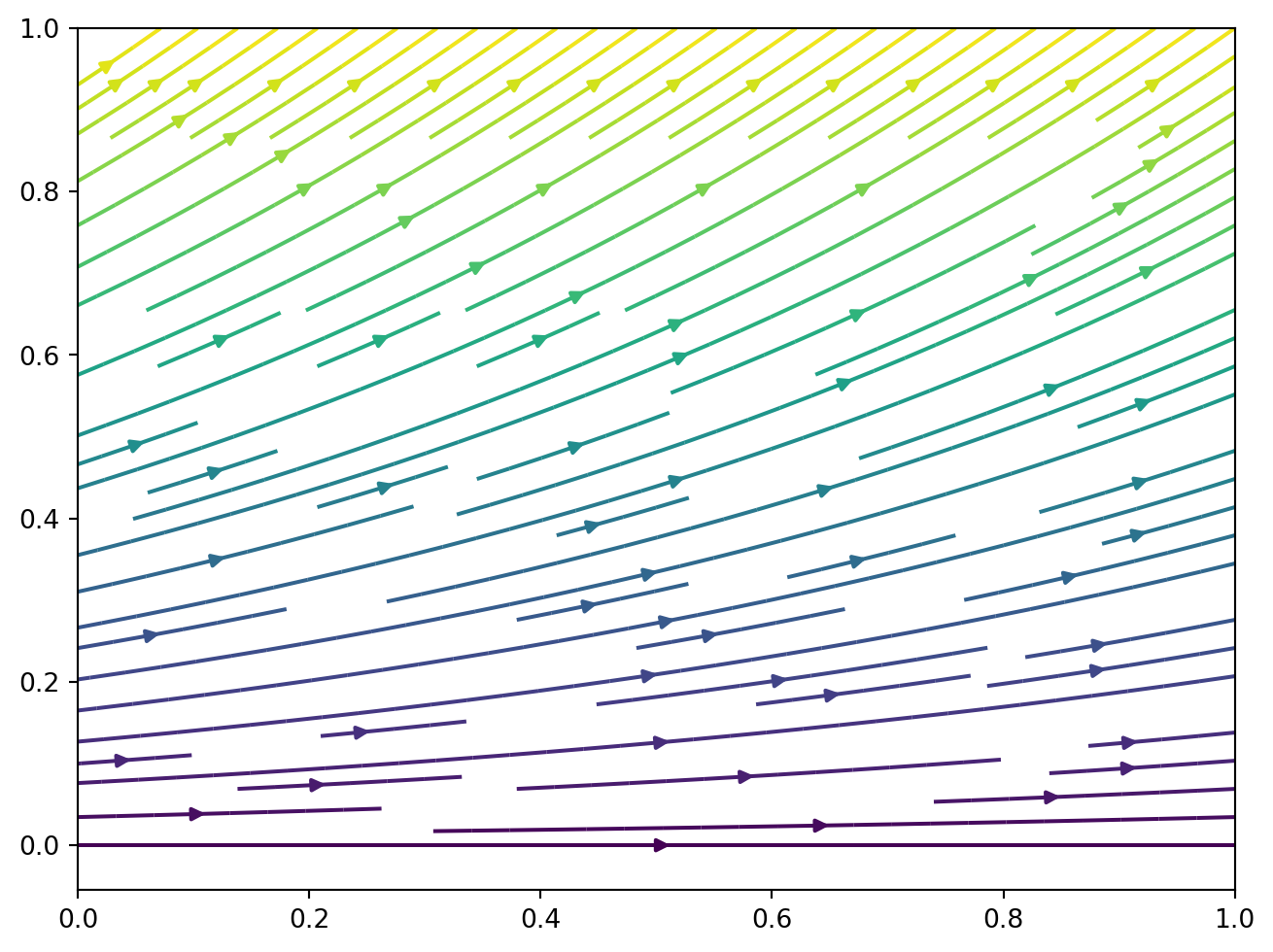
Vector-flow visualization is handled by BARBS, QUIVER, and STREAMPLOT. BARBS emphasizes meteorological-style wind encoding with flags and barbs, QUIVER gives direct arrow glyphs for sampled vectors, and STREAMPLOT traces continuous flow lines across a grid. Together they cover complementary views of velocity fields, electric fields, and gradient-driven transport. Typical use cases include checking boundary behavior in CFD outputs, comparing directional regimes across domains, and presenting motion patterns for technical reviews.
Scalar-field and surface-like rendering is provided by CONTOUR, CONTOUR_FILLED, and PCOLORMESH. CONTOUR isolates equal-value lines to reveal topology and critical regions, while CONTOUR_FILLED fills level bands to emphasize magnitude zones. PCOLORMESH maps cellwise values directly, which is useful when grid resolution or discontinuities should remain visible. These functions are commonly used for temperature maps, pressure distributions, concentration fields, and simulation snapshots where both local variation and global structure matter.
Logarithmic and scale-transform analysis is covered by LOGLOG, SEMILOGX, and SEMILOGY. LOGLOG is useful for power-law behavior where straight lines imply y\propto x^m, while SEMILOGX and SEMILOGY separate exponential-like effects along one axis at a time. In practice, these charts support model linearization checks, calibration curve interpretation, and order-of-magnitude comparisons. They are especially valuable when measurements span decades and linear axes would compress important variation.
Non-Cartesian and multivariate profile views are offered by POLAR_LINE, POLAR_SCATTER, POLAR_BAR, and RADAR. The three polar functions use angle-radius coordinates for directional intensity, periodic signals, and orientation-dependent measurements. RADAR summarizes multiple variables around a circular axis to compare entities across shared dimensions. These tools are frequently applied in cyclic sensor analysis, bearing-based phenomena, and compact scorecard-style technical comparisons.
Triangulation-based irregular-mesh plotting is addressed by TRIPLOT, TRICONTOUR, TRICONTOUR_FILLED, and TRIPCOLOR. TRIPLOT exposes mesh connectivity, TRICONTOUR and TRICONTOUR_FILLED compute contour structure on unstructured points, and TRIPCOLOR provides direct face/vertex color mapping. This group is essential for finite-element style datasets, scattered spatial observations, and domains where structured grids are not available. Used together, they support both mesh-quality diagnostics and field interpretation on complex geometries.
BARBS
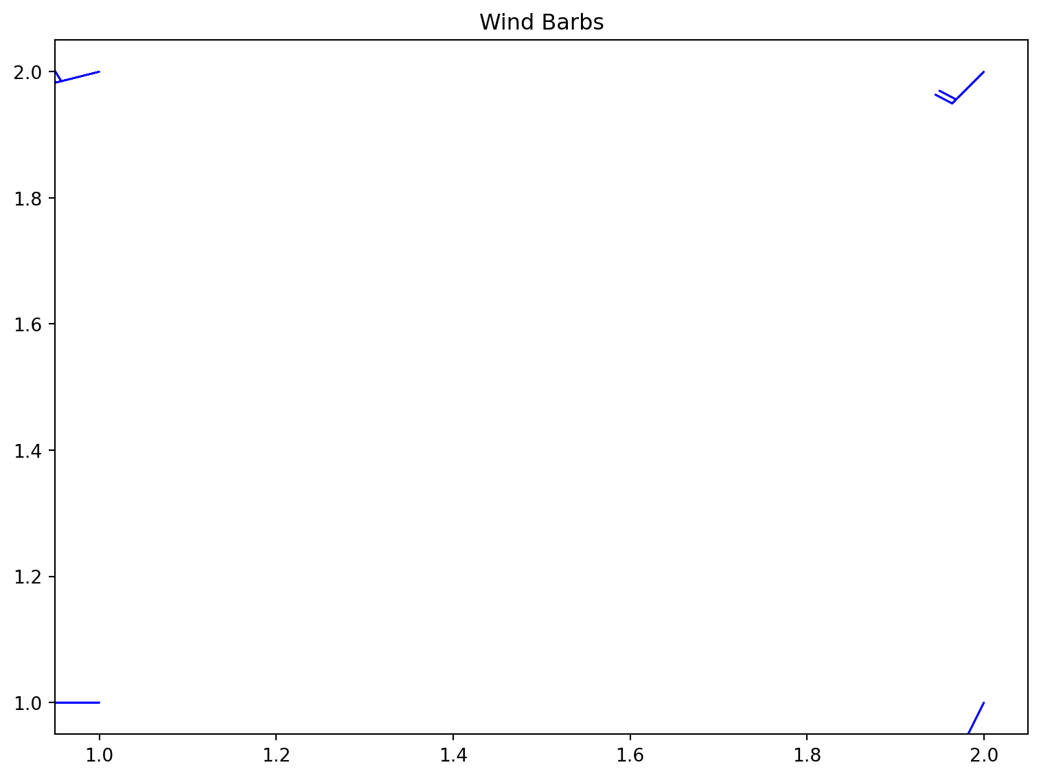
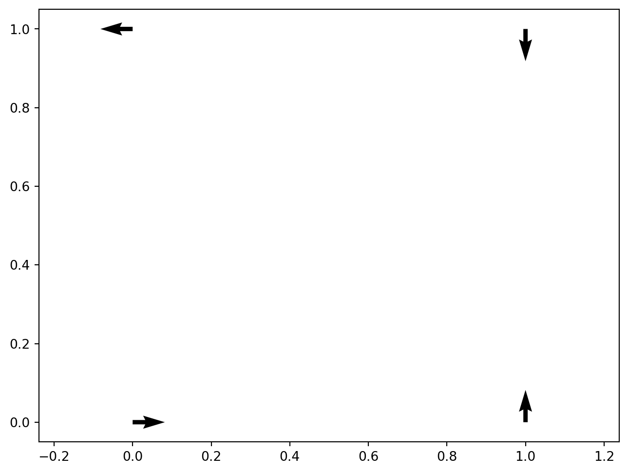
Plot a 2D field of wind barbs.
Excel Usage
=BARBS(data, title, xlabel, ylabel, barb_color)data(list[list], required): Input data with 4 columns (X, Y, U, V).title(str, optional, default: null): Chart title.xlabel(str, optional, default: null): Label for X-axis.ylabel(str, optional, default: null): Label for Y-axis.barb_color(str, optional, default: “blue”): Color of the barbs.
Returns (object): Matplotlib Figure object (standard Python) or base64 encoded PNG string (Pyodide).
Example 1: Simple wind barb field
Inputs:
| data | title | |||
|---|---|---|---|---|
| 1 | 1 | 10 | 0 | Wind Barbs |
| 1 | 2 | 20 | 5 | |
| 2 | 1 | 5 | 10 | |
| 2 | 2 | 15 | 15 |
Excel formula:
=BARBS({1,1,10,0;1,2,20,5;2,1,5,10;2,2,15,15}, "Wind Barbs")Expected output:
"chart"
Example 2: Green wind barbs
Inputs:
| data | barb_color | |||
|---|---|---|---|---|
| 1 | 1 | 10 | 10 | green |
| 2 | 2 | 20 | 20 |
Excel formula:
=BARBS({1,1,10,10;2,2,20,20}, "green")Expected output:
"chart"
Example 3: Red wind barbs with labels
Inputs:
| data | barb_color | xlabel | ylabel | |||
|---|---|---|---|---|---|---|
| 0 | 0 | 5 | 5 | red | East | North |
| 1 | 1 | 15 | 15 |
Excel formula:
=BARBS({0,0,5,5;1,1,15,15}, "red", "East", "North")Expected output:
"chart"
Example 4: Black wind barbs
Inputs:
| data | barb_color | |||
|---|---|---|---|---|
| 0 | 0 | 30 | 0 | black |
| 0 | 1 | 0 | 30 |
Excel formula:
=BARBS({0,0,30,0;0,1,0,30}, "black")Expected output:
"chart"
Python Code
Show Code
import sys
import matplotlib
IS_PYODIDE = sys.platform == "emscripten"
if IS_PYODIDE:
    matplotlib.use('Agg')
import matplotlib.pyplot as plt
import io
import base64
import numpy as np

def barbs(data, title=None, xlabel=None, ylabel=None, barb_color='blue'):
    """
    Plot a 2D field of wind barbs.

    See: https://matplotlib.org/stable/api/_as_gen/matplotlib.axes.Axes.barbs.html

    This example function is provided as-is without any representation of accuracy.

    Args:
        data (list[list]): Input data with 4 columns (X, Y, U, V).
        title (str, optional): Chart title. Default is None.
        xlabel (str, optional): Label for X-axis. Default is None.
        ylabel (str, optional): Label for Y-axis. Default is None.
        barb_color (str, optional): Color of the barbs. Valid options: Blue, Green, Red, Black. Default is 'blue'.

    Returns:
        object: Matplotlib Figure object (standard Python) or base64 encoded PNG string (Pyodide).
    """
    def to2d(x):
        return [[x]] if not isinstance(x, list) else x

    try:
        data = to2d(data)
        if not isinstance(data, list) or not data or not isinstance(data[0], list):
            return "Error: Input data must be a 2D list."

        # Convert to numpy array
        try:
            arr = np.array(data, dtype=float)
        except Exception:
            return "Error: Data must be numeric."

        if arr.shape[1] < 4:
            return "Error: Data must have at least 4 columns (X, Y, U, V)."

        # Extract coordinates
        X, Y, U, V = arr[:, 0], arr[:, 1], arr[:, 2], arr[:, 3]

        # Create figure
        fig, ax = plt.subplots(figsize=(8, 6))

        # Plot barbs
        ax.barbs(X, Y, U, V, barbcolor=barb_color, flagcolor=barb_color)

        # Set labels and title
        if title:
            ax.set_title(title)
        if xlabel:
            ax.set_xlabel(xlabel)
        if ylabel:
            ax.set_ylabel(ylabel)

        plt.tight_layout()

        if IS_PYODIDE:
            buf = io.BytesIO()
            plt.savefig(buf, format='png', dpi=100, bbox_inches='tight')
            plt.close(fig)
            buf.seek(0)
            img_bytes = buf.read()
            img_b64 = base64.b64encode(img_bytes).decode('utf-8')
            return f"data:image/png;base64,{img_b64}"
        else:
            return fig
    except Exception as e:
        return f"Error: {str(e)}"
Online Calculator
Input data with 4 columns (X, Y, U, V).
Chart title.
Label for X-axis.
Label for Y-axis.
Color of the barbs.
CONTOUR
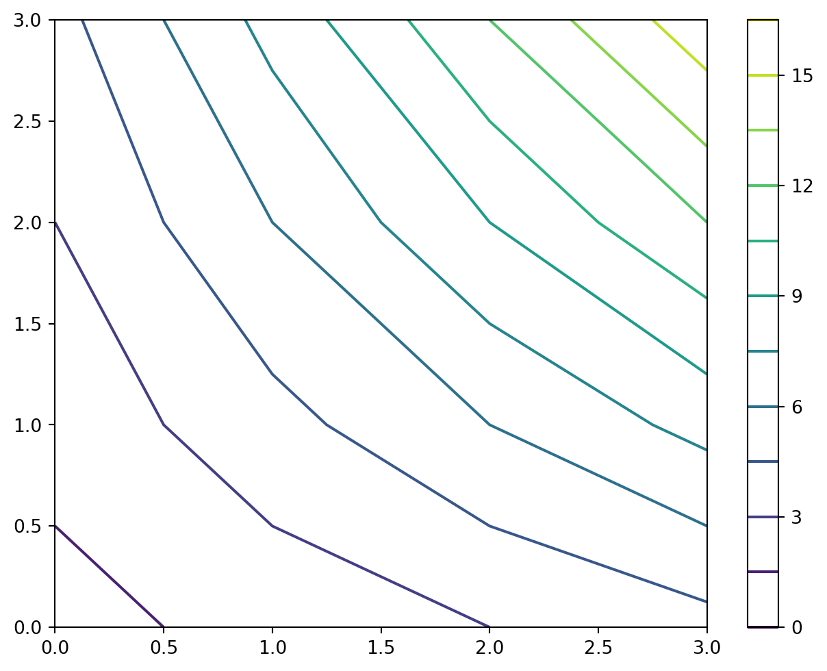
Create a contour plot.
Excel Usage
=CONTOUR(data, title, xlabel, ylabel, color_map, levels, colorbar)data(list[list], required): Input Z-data.title(str, optional, default: null): Chart title.xlabel(str, optional, default: null): Label for X-axis.ylabel(str, optional, default: null): Label for Y-axis.color_map(str, optional, default: “viridis”): Color map for contours.levels(int, optional, default: 10): Number of contour levels.colorbar(str, optional, default: “true”): Show colorbar.
Returns (object): Matplotlib Figure object (standard Python) or base64 encoded PNG string (Pyodide).
Example 1: Basic contour plot
Inputs:
| data | |||
|---|---|---|---|
| 1 | 2 | 3 | 4 |
| 2 | 4 | 6 | 8 |
| 3 | 6 | 9 | 12 |
| 4 | 8 | 12 | 16 |
Excel formula:
=CONTOUR({1,2,3,4;2,4,6,8;3,6,9,12;4,8,12,16})Expected output:
"chart"
Example 2: Contour with plasma colormap
Inputs:
| data | color_map | ||
|---|---|---|---|
| 0 | 1 | 2 | plasma |
| 1 | 2 | 3 | |
| 2 | 3 | 4 |
Excel formula:
=CONTOUR({0,1,2;1,2,3;2,3,4}, "plasma")Expected output:
"chart"
Example 3: Contour with axis labels and title
Inputs:
| data | title | xlabel | ylabel | ||
|---|---|---|---|---|---|
| 1 | 2 | 3 | Contour Plot | X | Y |
| 2 | 4 | 6 | |||
| 3 | 6 | 9 |
Excel formula:
=CONTOUR({1,2,3;2,4,6;3,6,9}, "Contour Plot", "X", "Y")Expected output:
"chart"
Example 4: Contour with 20 levels
Inputs:
| data | levels | ||||
|---|---|---|---|---|---|
| 1 | 2 | 3 | 4 | 5 | 20 |
| 2 | 3 | 4 | 5 | 6 | |
| 3 | 4 | 5 | 6 | 7 | |
| 4 | 5 | 6 | 7 | 8 |
Excel formula:
=CONTOUR({1,2,3,4,5;2,3,4,5,6;3,4,5,6,7;4,5,6,7,8}, 20)Expected output:
"chart"
Python Code
Show Code
import sys
import matplotlib
IS_PYODIDE = sys.platform == "emscripten"
if IS_PYODIDE:
    matplotlib.use('Agg')
import matplotlib.pyplot as plt
import io
import base64
import numpy as np

def contour(data, title=None, xlabel=None, ylabel=None, color_map='viridis', levels=10, colorbar='true'):
    """
    Create a contour plot.

    See: https://matplotlib.org/stable/api/_as_gen/matplotlib.pyplot.contour.html

    This example function is provided as-is without any representation of accuracy.

    Args:
        data (list[list]): Input Z-data.
        title (str, optional): Chart title. Default is None.
        xlabel (str, optional): Label for X-axis. Default is None.
        ylabel (str, optional): Label for Y-axis. Default is None.
        color_map (str, optional): Color map for contours. Valid options: Viridis, Plasma, Inferno, Magma, Cividis. Default is 'viridis'.
        levels (int, optional): Number of contour levels. Default is 10.
        colorbar (str, optional): Show colorbar. Valid options: True, False. Default is 'true'.

    Returns:
        object: Matplotlib Figure object (standard Python) or base64 encoded PNG string (Pyodide).
    """
    def to2d(x):
        return [[x]] if not isinstance(x, list) else x

    try:
        data = to2d(data)

        if not isinstance(data, list) or not all(isinstance(row, list) for row in data):
            return "Error: Invalid input - data must be a 2D list"

        # Convert to numpy array
        Z = []
        for row in data:
            z_row = []
            for val in row:
                try:
                    z_row.append(float(val))
                except (TypeError, ValueError):
                    z_row.append(0)
            Z.append(z_row)

        Z = np.array(Z)

        if Z.size == 0:
            return "Error: No valid data found"

        # Create X and Y coordinates
        rows, cols = Z.shape
        X = np.arange(cols)
        Y = np.arange(rows)
        X, Y = np.meshgrid(X, Y)

        # Create contour plot
        fig, ax = plt.subplots(figsize=(8, 6))

        CS = ax.contour(X, Y, Z, levels=levels, cmap=color_map)

        if colorbar == "true":
            plt.colorbar(CS, ax=ax)

        if title:
            ax.set_title(title)
        if xlabel:
            ax.set_xlabel(xlabel)
        if ylabel:
            ax.set_ylabel(ylabel)

        if IS_PYODIDE:
            buf = io.BytesIO()
            plt.savefig(buf, format='png', bbox_inches='tight')
            plt.close(fig)
            buf.seek(0)
            img_base64 = base64.b64encode(buf.read()).decode('utf-8')
            return f"data:image/png;base64,{img_base64}"
        else:
            return fig
    except Exception as e:
        return f"Error: {str(e)}"
Online Calculator
Input Z-data.
Chart title.
Label for X-axis.
Label for Y-axis.
Color map for contours.
Number of contour levels.
Show colorbar.
CONTOUR_FILLED
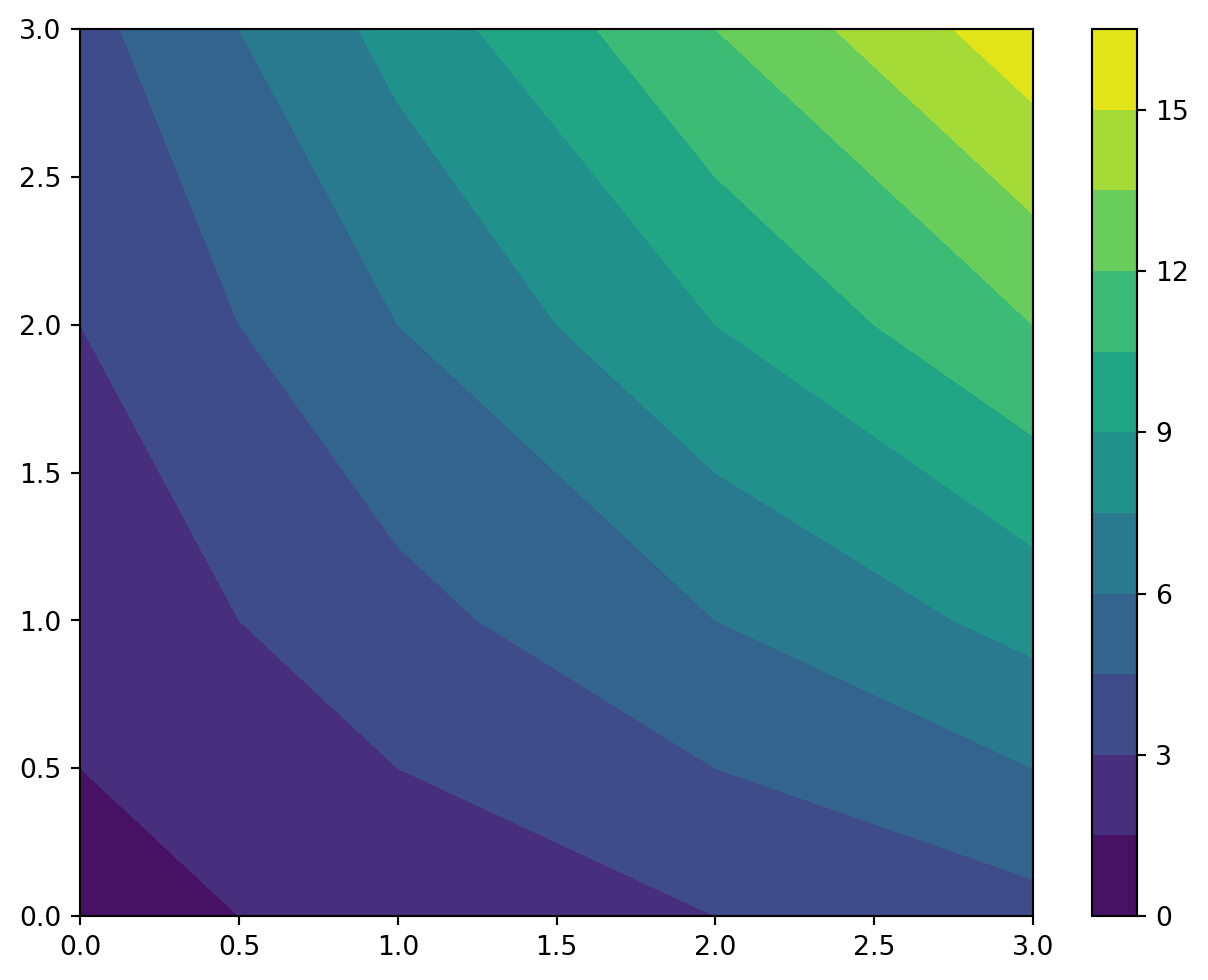
Create a filled contour plot.
Excel Usage
=CONTOUR_FILLED(data, title, xlabel, ylabel, color_map, levels, colorbar)data(list[list], required): Input Z-data.title(str, optional, default: null): Chart title.xlabel(str, optional, default: null): Label for X-axis.ylabel(str, optional, default: null): Label for Y-axis.color_map(str, optional, default: “viridis”): Color map for contours.levels(int, optional, default: 10): Number of contour levels.colorbar(str, optional, default: “true”): Show colorbar.
Returns (object): Matplotlib Figure object (standard Python) or base64 encoded PNG string (Pyodide).
Example 1: Basic filled contour plot
Inputs:
| data | |||
|---|---|---|---|
| 1 | 2 | 3 | 4 |
| 2 | 4 | 6 | 8 |
| 3 | 6 | 9 | 12 |
| 4 | 8 | 12 | 16 |
Excel formula:
=CONTOUR_FILLED({1,2,3,4;2,4,6,8;3,6,9,12;4,8,12,16})Expected output:
"chart"
Example 2: Filled contour with inferno colormap
Inputs:
| data | color_map | ||
|---|---|---|---|
| 0 | 1 | 2 | inferno |
| 1 | 2 | 3 | |
| 2 | 3 | 4 |
Excel formula:
=CONTOUR_FILLED({0,1,2;1,2,3;2,3,4}, "inferno")Expected output:
"chart"
Example 3: Filled contour with labels and title
Inputs:
| data | title | xlabel | ylabel | ||
|---|---|---|---|---|---|
| 1 | 2 | 3 | Filled Contour | X-axis | Y-axis |
| 2 | 4 | 6 | |||
| 3 | 6 | 9 |
Excel formula:
=CONTOUR_FILLED({1,2,3;2,4,6;3,6,9}, "Filled Contour", "X-axis", "Y-axis")Expected output:
"chart"
Example 4: Filled contour without colorbar
Inputs:
| data | colorbar | ||||
|---|---|---|---|---|---|
| 1 | 2 | 3 | 4 | 5 | false |
| 2 | 3 | 4 | 5 | 6 | |
| 3 | 4 | 5 | 6 | 7 |
Excel formula:
=CONTOUR_FILLED({1,2,3,4,5;2,3,4,5,6;3,4,5,6,7}, "false")Expected output:
"chart"
Python Code
Show Code
import sys
import matplotlib
IS_PYODIDE = sys.platform == "emscripten"
if IS_PYODIDE:
    matplotlib.use('Agg')
import matplotlib.pyplot as plt
import io
import base64
import numpy as np

def contour_filled(data, title=None, xlabel=None, ylabel=None, color_map='viridis', levels=10, colorbar='true'):
    """
    Create a filled contour plot.

    See: https://matplotlib.org/stable/api/_as_gen/matplotlib.pyplot.contourf.html

    This example function is provided as-is without any representation of accuracy.

    Args:
        data (list[list]): Input Z-data.
        title (str, optional): Chart title. Default is None.
        xlabel (str, optional): Label for X-axis. Default is None.
        ylabel (str, optional): Label for Y-axis. Default is None.
        color_map (str, optional): Color map for contours. Valid options: Viridis, Plasma, Inferno, Magma, Cividis. Default is 'viridis'.
        levels (int, optional): Number of contour levels. Default is 10.
        colorbar (str, optional): Show colorbar. Valid options: True, False. Default is 'true'.

    Returns:
        object: Matplotlib Figure object (standard Python) or base64 encoded PNG string (Pyodide).
    """
    def to2d(x):
        return [[x]] if not isinstance(x, list) else x

    try:
        data = to2d(data)

        if not isinstance(data, list) or not all(isinstance(row, list) for row in data):
            return "Error: Invalid input - data must be a 2D list"

        # Convert to numpy array
        Z = []
        for row in data:
            z_row = []
            for val in row:
                try:
                    z_row.append(float(val))
                except (TypeError, ValueError):
                    z_row.append(0)
            Z.append(z_row)

        Z = np.array(Z)

        if Z.size == 0:
            return "Error: No valid data found"

        # Create X and Y coordinates
        rows, cols = Z.shape
        X = np.arange(cols)
        Y = np.arange(rows)
        X, Y = np.meshgrid(X, Y)

        # Create filled contour plot
        fig, ax = plt.subplots(figsize=(8, 6))

        CS = ax.contourf(X, Y, Z, levels=levels, cmap=color_map)

        if colorbar == "true":
            plt.colorbar(CS, ax=ax)

        if title:
            ax.set_title(title)
        if xlabel:
            ax.set_xlabel(xlabel)
        if ylabel:
            ax.set_ylabel(ylabel)

        if IS_PYODIDE:
            buf = io.BytesIO()
            plt.savefig(buf, format='png', bbox_inches='tight')
            plt.close(fig)
            buf.seek(0)
            img_base64 = base64.b64encode(buf.read()).decode('utf-8')
            return f"data:image/png;base64,{img_base64}"
        else:
            return fig
    except Exception as e:
        return f"Error: {str(e)}"
Online Calculator
Input Z-data.
Chart title.
Label for X-axis.
Label for Y-axis.
Color map for contours.
Number of contour levels.
Show colorbar.
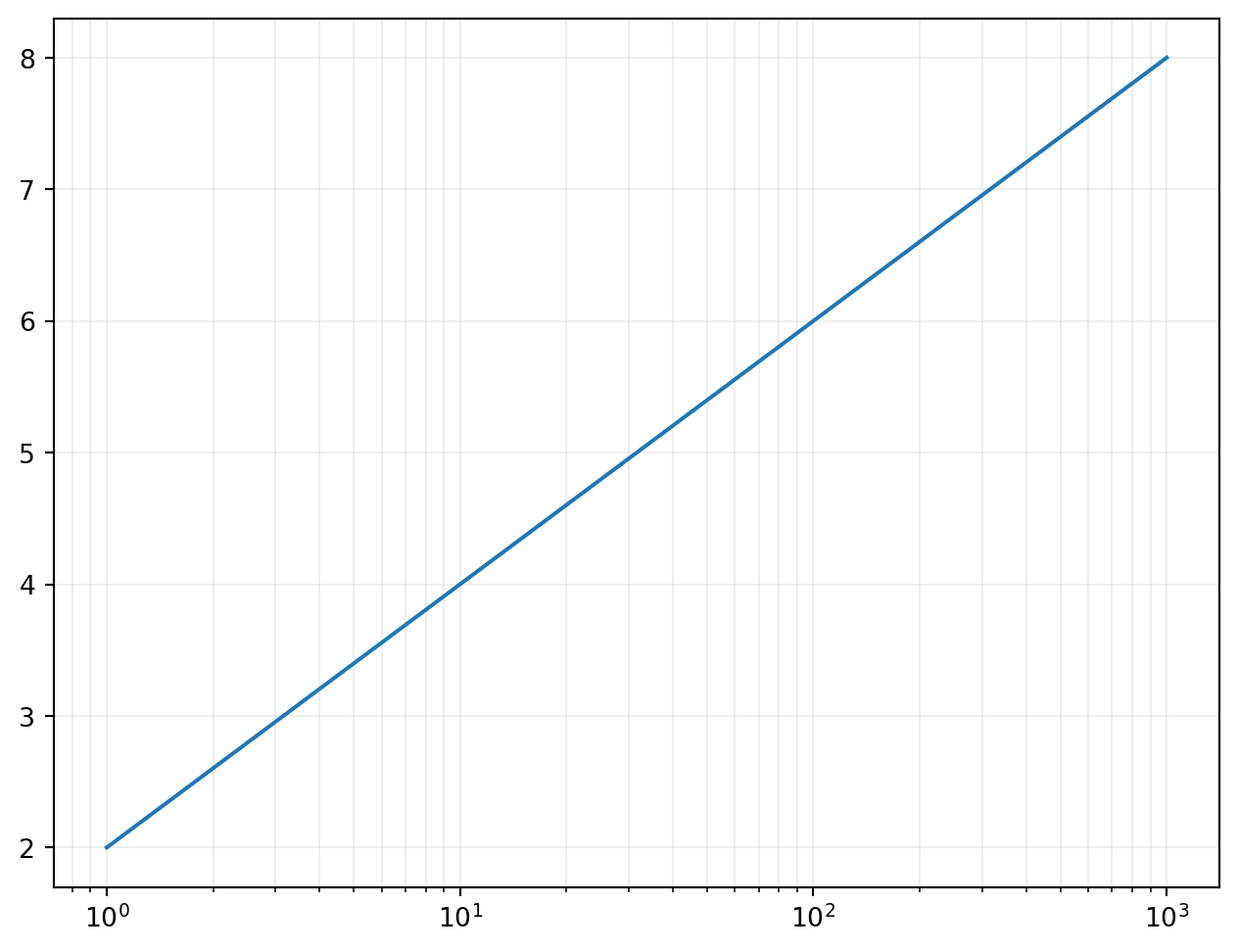
LOGLOG
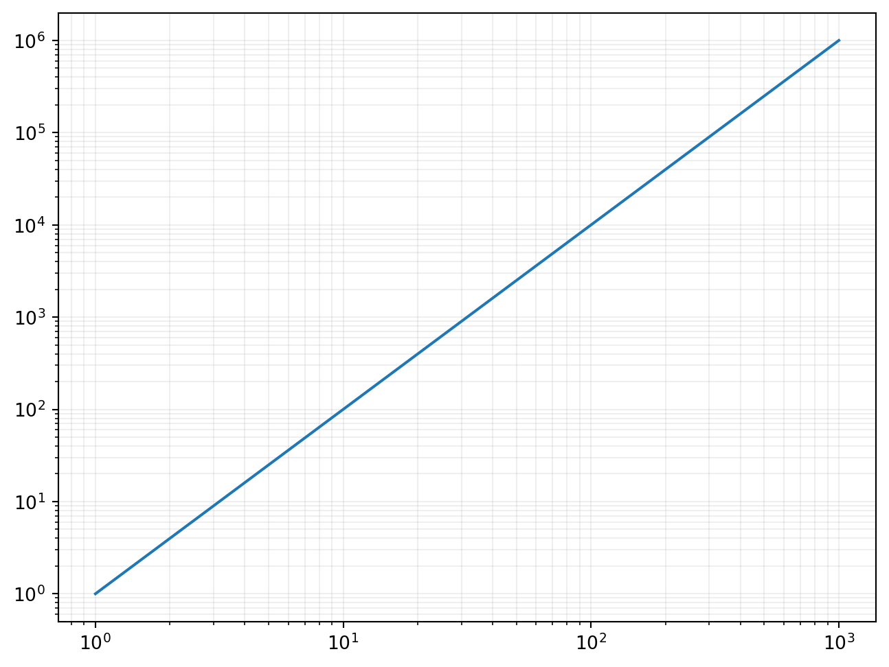
Create a log-log plot from data.
Excel Usage
=LOGLOG(data, title, xlabel, ylabel, plot_color, linestyle, marker, legend)data(list[list], required): Input data.title(str, optional, default: null): Chart title.xlabel(str, optional, default: null): Label for X-axis.ylabel(str, optional, default: null): Label for Y-axis.plot_color(str, optional, default: null): Line color.linestyle(str, optional, default: “-”): Line style (e.g., ‘-’, ‘–’).marker(str, optional, default: null): Marker style.legend(str, optional, default: “false”): Show legend.
Returns (object): Matplotlib Figure object (standard Python) or base64 encoded PNG string (Pyodide).
Example 1: Basic log-log plot
Inputs:
| data | |
|---|---|
| 1 | 1 |
| 10 | 100 |
| 100 | 10000 |
| 1000 | 1000000 |
Excel formula:
=LOGLOG({1,1;10,100;100,10000;1000,1000000})Expected output:
"chart"
Example 2: Log-log plot with multiple series
Inputs:
| data | legend | ||
|---|---|---|---|
| 1 | 1 | 2 | true |
| 10 | 100 | 50 | |
| 100 | 10000 | 5000 |
Excel formula:
=LOGLOG({1,1,2;10,100,50;100,10000,5000}, "true")Expected output:
"chart"
Example 3: Log-log plot with markers and color
Inputs:
| data | plot_color | marker | |
|---|---|---|---|
| 1 | 2 | red | o |
| 10 | 20 | ||
| 100 | 200 | ||
| 1000 | 2000 |
Excel formula:
=LOGLOG({1,2;10,20;100,200;1000,2000}, "red", "o")Expected output:
"chart"
Example 4: Log-log plot with labels and title
Inputs:
| data | title | xlabel | ylabel | |
|---|---|---|---|---|
| 1 | 1 | Log-Log | X (log) | Y (log) |
| 10 | 10 | |||
| 100 | 100 | |||
| 1000 | 1000 |
Excel formula:
=LOGLOG({1,1;10,10;100,100;1000,1000}, "Log-Log", "X (log)", "Y (log)")Expected output:
"chart"
Python Code
Show Code
import sys
import matplotlib
IS_PYODIDE = sys.platform == "emscripten"
if IS_PYODIDE:
    matplotlib.use('Agg')
import matplotlib.pyplot as plt
import io
import base64
import numpy as np

def loglog(data, title=None, xlabel=None, ylabel=None, plot_color=None, linestyle='-', marker=None, legend='false'):
    """
    Create a log-log plot from data.

    See: https://matplotlib.org/stable/api/_as_gen/matplotlib.pyplot.loglog.html

    This example function is provided as-is without any representation of accuracy.

    Args:
        data (list[list]): Input data.
        title (str, optional): Chart title. Default is None.
        xlabel (str, optional): Label for X-axis. Default is None.
        ylabel (str, optional): Label for Y-axis. Default is None.
        plot_color (str, optional): Line color. Valid options: Blue, Green, Red, Cyan, Magenta, Yellow, Black, White. Default is None.
        linestyle (str, optional): Line style (e.g., '-', '--'). Valid options: Solid, Dashed, Dotted, Dash-dot. Default is '-'.
        marker (str, optional): Marker style. Valid options: None, Point, Pixel, Circle, Square, Triangle Down, Triangle Up. Default is None.
        legend (str, optional): Show legend. Valid options: True, False. Default is 'false'.

    Returns:
        object: Matplotlib Figure object (standard Python) or base64 encoded PNG string (Pyodide).
    """
    def to2d(x):
        return [[x]] if not isinstance(x, list) else x

    try:
        data = to2d(data)

        if not isinstance(data, list) or not all(isinstance(row, list) for row in data):
            return "Error: Invalid input - data must be a 2D list"

        # Extract X and Y columns
        if len(data) < 1 or len(data[0]) < 2:
            return "Error: Data must have at least 2 columns"

        # Determine number of series (first column is X, rest are Y series)
        num_series = len(data[0]) - 1

        X = []
        Y_series = [[] for _ in range(num_series)]

        for row in data:
            if len(row) >= 2:
                try:
                    x_val = float(row[0])
                    if x_val > 0:  # Log scale requires positive values
                        X.append(x_val)
                        for i in range(num_series):
                            if i + 1 < len(row):
                                try:
                                    y_val = float(row[i + 1])
                                    if y_val > 0:
                                        Y_series[i].append(y_val)
                                    else:
                                        Y_series[i].append(None)
                                except (TypeError, ValueError):
                                    Y_series[i].append(None)
                            else:
                                Y_series[i].append(None)
                except (TypeError, ValueError):
                    continue

        if len(X) == 0:
            return "Error: No valid positive numeric data found"

        # Create log-log plot
        fig, ax = plt.subplots(figsize=(8, 6))

        # Plot each series
        for i, Y in enumerate(Y_series):
            plot_kwargs = {'linestyle': linestyle}
            if plot_color:
                plot_kwargs['color'] = plot_color
            if marker:
                plot_kwargs['marker'] = marker

            # Filter out None values
            X_filtered = [X[j] for j in range(len(X)) if j < len(Y) and Y[j] is not None]
            Y_filtered = [y for y in Y if y is not None]

            if len(X_filtered) > 0:
                ax.loglog(X_filtered, Y_filtered, label=f"Series {i+1}", **plot_kwargs)

        if title:
            ax.set_title(title)
        if xlabel:
            ax.set_xlabel(xlabel)
        if ylabel:
            ax.set_ylabel(ylabel)

        if legend == "true" and num_series > 1:
            ax.legend()

        ax.grid(True, which="both", ls="-", alpha=0.2)

        if IS_PYODIDE:
            buf = io.BytesIO()
            plt.savefig(buf, format='png', bbox_inches='tight')
            plt.close(fig)
            buf.seek(0)
            img_base64 = base64.b64encode(buf.read()).decode('utf-8')
            return f"data:image/png;base64,{img_base64}"
        else:
            return fig
    except Exception as e:
        return f"Error: {str(e)}"
Online Calculator
Input data.
Chart title.
Label for X-axis.
Label for Y-axis.
Line color.
Line style (e.g., '-', '--').
Marker style.
Show legend.
PCOLORMESH
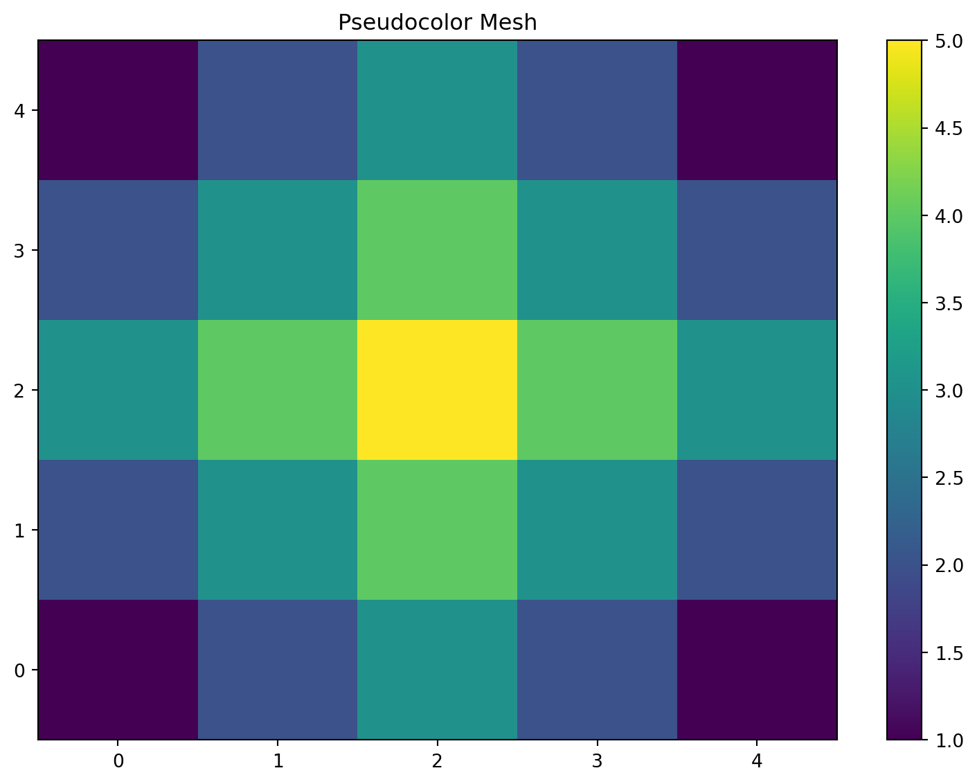
Create a pseudocolor plot with a rectangular grid.
Excel Usage
=PCOLORMESH(data, title, xlabel, ylabel, color_map, colorbar)data(list[list], required): 2D array of intensity values (Z).title(str, optional, default: null): Chart title.xlabel(str, optional, default: null): Label for X-axis.ylabel(str, optional, default: null): Label for Y-axis.color_map(str, optional, default: “viridis”): Color map.colorbar(str, optional, default: “true”): Show colorbar.
Returns (object): Matplotlib Figure object (standard Python) or base64 encoded PNG string (Pyodide).
Example 1: Basic 5x5 pseudocolor mesh
Inputs:
| data | title | ||||
|---|---|---|---|---|---|
| 1 | 2 | 3 | 2 | 1 | Pseudocolor Mesh |
| 2 | 3 | 4 | 3 | 2 | |
| 3 | 4 | 5 | 4 | 3 | |
| 2 | 3 | 4 | 3 | 2 | |
| 1 | 2 | 3 | 2 | 1 |
Excel formula:
=PCOLORMESH({1,2,3,2,1;2,3,4,3,2;3,4,5,4,3;2,3,4,3,2;1,2,3,2,1}, "Pseudocolor Mesh")Expected output:
"chart"
Example 2: Mesh with magma colormap
Inputs:
| data | color_map | ||
|---|---|---|---|
| 1 | 5 | 2 | magma |
| 4 | 2 | 6 |
Excel formula:
=PCOLORMESH({1,5,2;4,2,6}, "magma")Expected output:
"chart"
Example 3: Mesh without colorbar
Inputs:
| data | colorbar | |
|---|---|---|
| 1 | 1 | false |
| 1 | 1 |
Excel formula:
=PCOLORMESH({1,1;1,1}, "false")Expected output:
"chart"
Example 4: Mesh with cividis colormap
Inputs:
| data | color_map | |
|---|---|---|
| 1 | 2 | cividis |
| 3 | 4 |
Excel formula:
=PCOLORMESH({1,2;3,4}, "cividis")Expected output:
"chart"
Python Code
Show Code
import sys
import matplotlib
IS_PYODIDE = sys.platform == "emscripten"
if IS_PYODIDE:
    matplotlib.use('Agg')
import matplotlib.pyplot as plt
import io
import base64
import numpy as np

def pcolormesh(data, title=None, xlabel=None, ylabel=None, color_map='viridis', colorbar='true'):
    """
    Create a pseudocolor plot with a rectangular grid.

    See: https://matplotlib.org/stable/api/_as_gen/matplotlib.pyplot.pcolormesh.html

    This example function is provided as-is without any representation of accuracy.

    Args:
        data (list[list]): 2D array of intensity values (Z).
        title (str, optional): Chart title. Default is None.
        xlabel (str, optional): Label for X-axis. Default is None.
        ylabel (str, optional): Label for Y-axis. Default is None.
        color_map (str, optional): Color map. Valid options: Viridis, Plasma, Inferno, Magma, Cividis. Default is 'viridis'.
        colorbar (str, optional): Show colorbar. Valid options: True, False. Default is 'true'.

    Returns:
        object: Matplotlib Figure object (standard Python) or base64 encoded PNG string (Pyodide).
    """
    def to2d(x):
        return [[x]] if not isinstance(x, list) else x

    try:
        data = to2d(data)
        if not isinstance(data, list) or not data or not isinstance(data[0], list):
            return "Error: Input data must be a 2D list."

        # Convert to numpy array
        try:
            Z = np.array(data, dtype=float)
        except Exception:
            return "Error: Data must be numeric."

        if Z.ndim != 2:
            return "Error: Data must be a 2D array (matrix)."

        # Create X and Y coordinates (regular grid inferred from Z)
        rows, cols = Z.shape
        X, Y = np.meshgrid(np.arange(cols), np.arange(rows))

        # Create figure
        fig, ax = plt.subplots(figsize=(8, 6))

        # Plot pcolormesh
        im = ax.pcolormesh(X, Y, Z, cmap=color_map, shading='auto')

        # Add colorbar if requested
        if colorbar == "true":
            plt.colorbar(im, ax=ax)

        # Set labels and title
        if title:
            ax.set_title(title)
        if xlabel:
            ax.set_xlabel(xlabel)
        if ylabel:
            ax.set_ylabel(ylabel)

        plt.tight_layout()

        if IS_PYODIDE:
            buf = io.BytesIO()
            plt.savefig(buf, format='png', dpi=100, bbox_inches='tight')
            plt.close(fig)
            buf.seek(0)
            img_bytes = buf.read()
            img_b64 = base64.b64encode(img_bytes).decode('utf-8')
            return f"data:image/png;base64,{img_b64}"
        else:
            return fig
    except Exception as e:
        return f"Error: {str(e)}"
Online Calculator
2D array of intensity values (Z).
Chart title.
Label for X-axis.
Label for Y-axis.
Color map.
Show colorbar.
POLAR_BAR
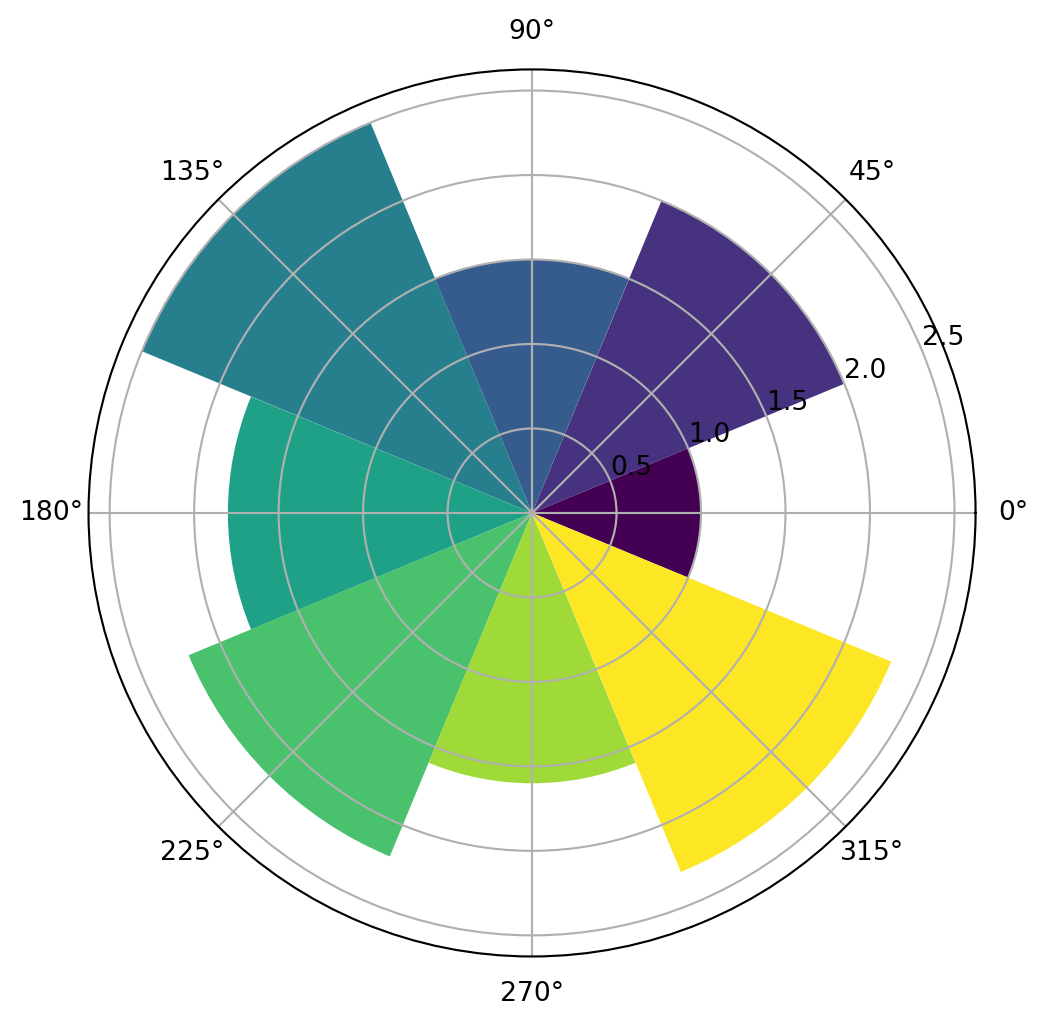
Create a bar chart in polar coordinates (also known as a Rose diagram).
Excel Usage
=POLAR_BAR(data, title, color_map, bottom, legend)data(list[list], required): Input data (Theta, R).title(str, optional, default: null): Chart title.color_map(str, optional, default: “viridis”): Color map for bars.bottom(float, optional, default: 0): Base of the bars.legend(str, optional, default: “false”): Show legend.
Returns (object): Matplotlib Figure object (standard Python) or base64 encoded PNG string (Pyodide).
Example 1: Basic polar bar (rose diagram)
Inputs:
| data | |
|---|---|
| 0 | 1 |
| 0.785 | 2 |
| 1.571 | 1.5 |
| 2.356 | 2.5 |
| 3.142 | 1.8 |
| 3.927 | 2.2 |
| 4.712 | 1.6 |
| 5.498 | 2.3 |
Excel formula:
=POLAR_BAR({0,1;0.785,2;1.571,1.5;2.356,2.5;3.142,1.8;3.927,2.2;4.712,1.6;5.498,2.3})Expected output:
"chart"
Example 2: Polar bar with plasma colormap
Inputs:
| data | color_map | |
|---|---|---|
| 0 | 1.5 | plasma |
| 1.047 | 2.5 | |
| 2.094 | 3 | |
| 3.142 | 2 | |
| 4.189 | 2.8 | |
| 5.236 | 1.8 |
Excel formula:
=POLAR_BAR({0,1.5;1.047,2.5;2.094,3;3.142,2;4.189,2.8;5.236,1.8}, "plasma")Expected output:
"chart"
Example 3: Polar bar with offset bottom
Inputs:
| data | bottom | |
|---|---|---|
| 0 | 2 | 1 |
| 1.571 | 3 | |
| 3.142 | 2.5 | |
| 4.712 | 3.5 |
Excel formula:
=POLAR_BAR({0,2;1.571,3;3.142,2.5;4.712,3.5}, 1)Expected output:
"chart"
Example 4: Polar bar with title
Inputs:
| data | title | |
|---|---|---|
| 0 | 1 | Rose Diagram |
| 1.571 | 2 | |
| 3.142 | 1.5 | |
| 4.712 | 2.5 |
Excel formula:
=POLAR_BAR({0,1;1.571,2;3.142,1.5;4.712,2.5}, "Rose Diagram")Expected output:
"chart"
Python Code
Show Code
import sys
import matplotlib
IS_PYODIDE = sys.platform == "emscripten"
if IS_PYODIDE:
    matplotlib.use('Agg')
import matplotlib.pyplot as plt
import io
import base64
import numpy as np

def polar_bar(data, title=None, color_map='viridis', bottom=0, legend='false'):
    """
    Create a bar chart in polar coordinates (also known as a Rose diagram).

    See: https://matplotlib.org/stable/api/_as_gen/matplotlib.axes.Axes.bar.html

    This example function is provided as-is without any representation of accuracy.

    Args:
        data (list[list]): Input data (Theta, R).
        title (str, optional): Chart title. Default is None.
        color_map (str, optional): Color map for bars. Valid options: Viridis, Plasma, Inferno, Magma, Cividis. Default is 'viridis'.
        bottom (float, optional): Base of the bars. Default is 0.
        legend (str, optional): Show legend. Valid options: True, False. Default is 'false'.

    Returns:
        object: Matplotlib Figure object (standard Python) or base64 encoded PNG string (Pyodide).
    """
    def to2d(x):
        return [[x]] if not isinstance(x, list) else x

    try:
        data = to2d(data)

        if not isinstance(data, list) or not all(isinstance(row, list) for row in data):
            return "Error: Invalid input - data must be a 2D list"

        # Extract theta and r columns
        if len(data) < 1 or len(data[0]) < 2:
            return "Error: Data must have at least 2 columns (Theta, R)"

        theta = []
        r = []
        for row in data:
            if len(row) >= 2:
                try:
                    theta.append(float(row[0]))
                    r.append(float(row[1]))
                except (TypeError, ValueError):
                    continue

        if len(theta) == 0:
            return "Error: No valid numeric data found"

        # Calculate bar width
        if len(theta) > 1:
            width = 2 * np.pi / len(theta)
        else:
            width = 0.5

        # Create polar plot
        fig = plt.figure(figsize=(8, 6))
        ax = fig.add_subplot(111, projection='polar')

        # Create colors from colormap
        cmap = plt.get_cmap(color_map)
        colors = cmap(np.linspace(0, 1, len(theta)))

        ax.bar(theta, r, width=width, bottom=bottom, color=colors)

        if title:
            ax.set_title(title)

        if legend == "true":
            ax.legend(['Data'])

        if IS_PYODIDE:
            buf = io.BytesIO()
            plt.savefig(buf, format='png', bbox_inches='tight')
            plt.close(fig)
            buf.seek(0)
            img_base64 = base64.b64encode(buf.read()).decode('utf-8')
            return f"data:image/png;base64,{img_base64}"
        else:
            return fig
    except Exception as e:
        return f"Error: {str(e)}"
Online Calculator
Input data (Theta, R).
Chart title.
Color map for bars.
Base of the bars.
Show legend.
POLAR_LINE
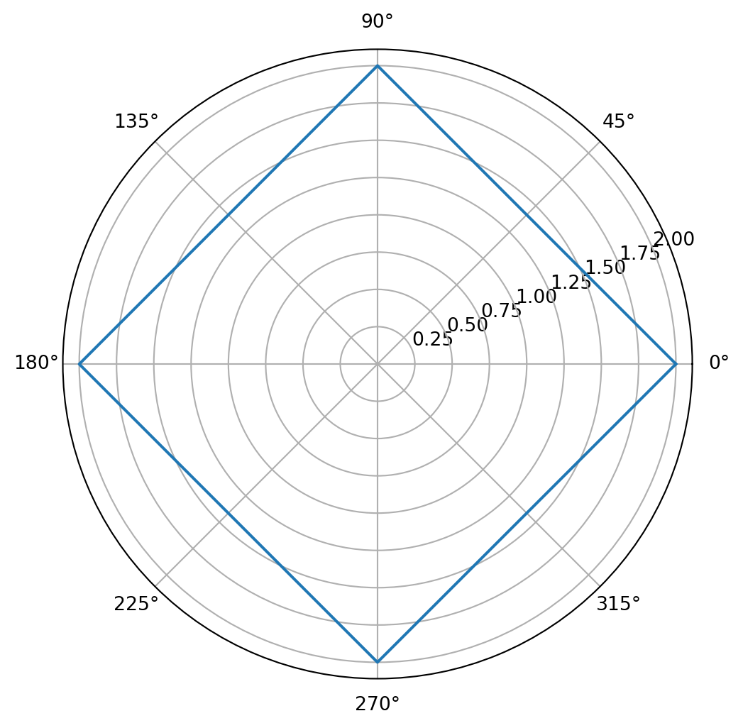
Create a line plot in polar coordinates.
Excel Usage
=POLAR_LINE(data, title, plot_color, linestyle, linewidth, legend)data(list[list], required): Input data (Theta, R).title(str, optional, default: null): Chart title.plot_color(str, optional, default: null): Line color.linestyle(str, optional, default: “-”): Line style (e.g., ‘-’, ‘–’).linewidth(float, optional, default: 1.5): Line width.legend(str, optional, default: “false”): Show legend.
Returns (object): Matplotlib Figure object (standard Python) or base64 encoded PNG string (Pyodide).
Example 1: Basic polar line forming a circle
Inputs:
| data | |
|---|---|
| 0 | 2 |
| 1.571 | 2 |
| 3.142 | 2 |
| 4.712 | 2 |
| 6.283 | 2 |
Excel formula:
=POLAR_LINE({0,2;1.571,2;3.142,2;4.712,2;6.283,2})Expected output:
"chart"
Example 2: Polar line with blue color and dashed style
Inputs:
| data | plot_color | linestyle | |
|---|---|---|---|
| 0 | 1 | blue | – |
| 0.785 | 1.5 | ||
| 1.571 | 2 | ||
| 2.356 | 2.5 | ||
| 3.142 | 3 |
Excel formula:
=POLAR_LINE({0,1;0.785,1.5;1.571,2;2.356,2.5;3.142,3}, "blue", "--")Expected output:
"chart"
Example 3: Polar line spiral pattern
Inputs:
| data | |
|---|---|
| 0 | 0.5 |
| 0.785 | 1 |
| 1.571 | 1.5 |
| 2.356 | 2 |
| 3.142 | 2.5 |
| 3.927 | 3 |
Excel formula:
=POLAR_LINE({0,0.5;0.785,1;1.571,1.5;2.356,2;3.142,2.5;3.927,3})Expected output:
"chart"
Example 4: Polar line with title and legend
Inputs:
| data | title | legend | |
|---|---|---|---|
| 0 | 1 | Polar Line | true |
| 1.571 | 2 | ||
| 3.142 | 1.5 | ||
| 4.712 | 2.5 |
Excel formula:
=POLAR_LINE({0,1;1.571,2;3.142,1.5;4.712,2.5}, "Polar Line", "true")Expected output:
"chart"
Python Code
Show Code
import sys
import matplotlib
IS_PYODIDE = sys.platform == "emscripten"
if IS_PYODIDE:
    matplotlib.use('Agg')
import matplotlib.pyplot as plt
import io
import base64
import numpy as np

def polar_line(data, title=None, plot_color=None, linestyle='-', linewidth=1.5, legend='false'):
    """
    Create a line plot in polar coordinates.

    See: https://matplotlib.org/stable/api/_as_gen/matplotlib.axes.Axes.plot.html

    This example function is provided as-is without any representation of accuracy.

    Args:
        data (list[list]): Input data (Theta, R).
        title (str, optional): Chart title. Default is None.
        plot_color (str, optional): Line color. Valid options: Blue, Green, Red, Cyan, Magenta, Yellow, Black, White. Default is None.
        linestyle (str, optional): Line style (e.g., '-', '--'). Valid options: Solid, Dashed, Dotted, Dash-dot. Default is '-'.
        linewidth (float, optional): Line width. Default is 1.5.
        legend (str, optional): Show legend. Valid options: True, False. Default is 'false'.

    Returns:
        object: Matplotlib Figure object (standard Python) or base64 encoded PNG string (Pyodide).
    """
    def to2d(x):
        return [[x]] if not isinstance(x, list) else x

    try:
        data = to2d(data)

        if not isinstance(data, list) or not all(isinstance(row, list) for row in data):
            return "Error: Invalid input - data must be a 2D list"

        # Extract theta and r columns
        if len(data) < 1 or len(data[0]) < 2:
            return "Error: Data must have at least 2 columns (Theta, R)"

        theta = []
        r = []
        for row in data:
            if len(row) >= 2:
                try:
                    theta.append(float(row[0]))
                    r.append(float(row[1]))
                except (TypeError, ValueError):
                    continue

        if len(theta) == 0:
            return "Error: No valid numeric data found"

        # Create polar plot
        fig = plt.figure(figsize=(8, 6))
        ax = fig.add_subplot(111, projection='polar')

        # Apply color if specified
        plot_kwargs = {'linestyle': linestyle, 'linewidth': linewidth}
        if plot_color:
            plot_kwargs['color'] = plot_color

        ax.plot(theta, r, **plot_kwargs)

        if title:
            ax.set_title(title)

        if legend == "true":
            ax.legend(['Data'])

        if IS_PYODIDE:
            buf = io.BytesIO()
            plt.savefig(buf, format='png', bbox_inches='tight')
            plt.close(fig)
            buf.seek(0)
            img_base64 = base64.b64encode(buf.read()).decode('utf-8')
            return f"data:image/png;base64,{img_base64}"
        else:
            return fig
    except Exception as e:
        return f"Error: {str(e)}"
Online Calculator
Input data (Theta, R).
Chart title.
Line color.
Line style (e.g., '-', '--').
Line width.
Show legend.
POLAR_SCATTER
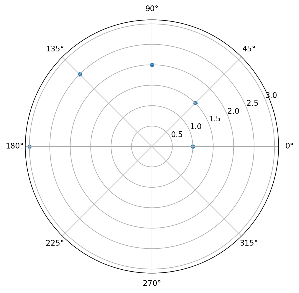
Create a scatter plot in polar coordinates.
Excel Usage
=POLAR_SCATTER(data, title, plot_color, marker, point_size, legend)data(list[list], required): Input data (Theta, R).title(str, optional, default: null): Chart title.plot_color(str, optional, default: null): Point color.marker(str, optional, default: “o”): Marker style.point_size(float, optional, default: 20): Size of points.legend(str, optional, default: “false”): Show legend.
Returns (object): Matplotlib Figure object (standard Python) or base64 encoded PNG string (Pyodide).
Example 1: Basic polar scatter spiral pattern
Inputs:
| data | |
|---|---|
| 0 | 1 |
| 0.785 | 1.5 |
| 1.571 | 2 |
| 2.356 | 2.5 |
| 3.142 | 3 |
Excel formula:
=POLAR_SCATTER({0,1;0.785,1.5;1.571,2;2.356,2.5;3.142,3})Expected output:
"chart"
Example 2: Polar scatter with red color
Inputs:
| data | plot_color | |
|---|---|---|
| 0 | 1 | red |
| 1.571 | 2 | |
| 3.142 | 1.5 | |
| 4.712 | 2.5 |
Excel formula:
=POLAR_SCATTER({0,1;1.571,2;3.142,1.5;4.712,2.5}, "red")Expected output:
"chart"
Example 3: Polar scatter with square markers
Inputs:
| data | marker | |
|---|---|---|
| 0 | 2 | s |
| 0.785 | 3 | |
| 1.571 | 2.5 | |
| 2.356 | 3.5 |
Excel formula:
=POLAR_SCATTER({0,2;0.785,3;1.571,2.5;2.356,3.5}, "s")Expected output:
"chart"
Example 4: Polar scatter with title and legend
Inputs:
| data | title | legend | |
|---|---|---|---|
| 0 | 1 | Polar Scatter | true |
| 1.571 | 2 | ||
| 3.142 | 3 |
Excel formula:
=POLAR_SCATTER({0,1;1.571,2;3.142,3}, "Polar Scatter", "true")Expected output:
"chart"
Python Code
Show Code
import sys
import matplotlib
IS_PYODIDE = sys.platform == "emscripten"
if IS_PYODIDE:
    matplotlib.use('Agg')
import matplotlib.pyplot as plt
import io
import base64
import numpy as np

def polar_scatter(data, title=None, plot_color=None, marker='o', point_size=20, legend='false'):
    """
    Create a scatter plot in polar coordinates.

    See: https://matplotlib.org/stable/api/_as_gen/matplotlib.axes.Axes.scatter.html

    This example function is provided as-is without any representation of accuracy.

    Args:
        data (list[list]): Input data (Theta, R).
        title (str, optional): Chart title. Default is None.
        plot_color (str, optional): Point color. Valid options: Blue, Green, Red, Cyan, Magenta, Yellow, Black, White. Default is None.
        marker (str, optional): Marker style. Valid options: None, Point, Pixel, Circle, Square, Triangle Down, Triangle Up. Default is 'o'.
        point_size (float, optional): Size of points. Default is 20.
        legend (str, optional): Show legend. Valid options: True, False. Default is 'false'.

    Returns:
        object: Matplotlib Figure object (standard Python) or base64 encoded PNG string (Pyodide).
    """
    def to2d(x):
        return [[x]] if not isinstance(x, list) else x

    try:
        data = to2d(data)

        if not isinstance(data, list) or not all(isinstance(row, list) for row in data):
            return "Error: Invalid input - data must be a 2D list"

        # Extract theta and r columns
        if len(data) < 1 or len(data[0]) < 2:
            return "Error: Data must have at least 2 columns (Theta, R)"

        theta = []
        r = []
        for row in data:
            if len(row) >= 2:
                try:
                    theta.append(float(row[0]))
                    r.append(float(row[1]))
                except (TypeError, ValueError):
                    continue

        if len(theta) == 0:
            return "Error: No valid numeric data found"

        # Create polar plot
        fig = plt.figure(figsize=(8, 6))
        ax = fig.add_subplot(111, projection='polar')

        # Apply color if specified
        scatter_kwargs = {'s': point_size}
        if plot_color:
            scatter_kwargs['color'] = plot_color

        ax.scatter(theta, r, marker=marker, **scatter_kwargs)

        if title:
            ax.set_title(title)

        if legend == "true":
            ax.legend(['Data'])

        if IS_PYODIDE:
            buf = io.BytesIO()
            plt.savefig(buf, format='png', bbox_inches='tight')
            plt.close(fig)
            buf.seek(0)
            img_base64 = base64.b64encode(buf.read()).decode('utf-8')
            return f"data:image/png;base64,{img_base64}"
        else:
            return fig
    except Exception as e:
        return f"Error: {str(e)}"
Online Calculator
Input data (Theta, R).
Chart title.
Point color.
Marker style.
Size of points.
Show legend.
QUIVER
Create a quiver plot (vector field arrows).
Excel Usage
=QUIVER(data, title, xlabel, ylabel, plot_color, scale)data(list[list], required): Input data (X, Y, U, V).title(str, optional, default: null): Chart title.xlabel(str, optional, default: null): Label for X-axis.ylabel(str, optional, default: null): Label for Y-axis.plot_color(str, optional, default: null): Arrow color.scale(float, optional, default: 1): Scaler for arrow length.
Returns (object): Matplotlib Figure object (standard Python) or base64 encoded PNG string (Pyodide).
Example 1: Basic quiver plot
Inputs:
| data | |||
|---|---|---|---|
| 0 | 0 | 1 | 0 |
| 1 | 0 | 0 | 1 |
| 0 | 1 | -1 | 0 |
| 1 | 1 | 0 | -1 |
Excel formula:
=QUIVER({0,0,1,0;1,0,0,1;0,1,-1,0;1,1,0,-1})Expected output:
"chart"
Example 2: Quiver plot with red arrows
Inputs:
| data | plot_color | |||
|---|---|---|---|---|
| 0 | 0 | 1 | 1 | red |
| 1 | 0 | -1 | 1 | |
| 0 | 1 | 1 | -1 | |
| 1 | 1 | -1 | -1 |
Excel formula:
=QUIVER({0,0,1,1;1,0,-1,1;0,1,1,-1;1,1,-1,-1}, "red")Expected output:
"chart"
Example 3: Quiver plot with labels and title
Inputs:
| data | title | xlabel | ylabel | |||
|---|---|---|---|---|---|---|
| 0 | 0 | 1 | 0 | Vector Field | X | Y |
| 1 | 0 | 0 | 1 | |||
| 2 | 0 | -1 | 0 |
Excel formula:
=QUIVER({0,0,1,0;1,0,0,1;2,0,-1,0}, "Vector Field", "X", "Y")Expected output:
"chart"
Example 4: Quiver plot with custom scale
Inputs:
| data | scale | |||
|---|---|---|---|---|
| 0 | 0 | 2 | 2 | 5 |
| 1 | 1 | -2 | 2 | |
| 2 | 0 | -2 | -2 |
Excel formula:
=QUIVER({0,0,2,2;1,1,-2,2;2,0,-2,-2}, 5)Expected output:
"chart"
Python Code
Show Code
import sys
import matplotlib
IS_PYODIDE = sys.platform == "emscripten"
if IS_PYODIDE:
    matplotlib.use('Agg')
import matplotlib.pyplot as plt
import io
import base64
import numpy as np

def quiver(data, title=None, xlabel=None, ylabel=None, plot_color=None, scale=1):
    """
    Create a quiver plot (vector field arrows).

    See: https://matplotlib.org/stable/api/_as_gen/matplotlib.pyplot.quiver.html

    This example function is provided as-is without any representation of accuracy.

    Args:
        data (list[list]): Input data (X, Y, U, V).
        title (str, optional): Chart title. Default is None.
        xlabel (str, optional): Label for X-axis. Default is None.
        ylabel (str, optional): Label for Y-axis. Default is None.
        plot_color (str, optional): Arrow color. Valid options: Blue, Green, Red, Cyan, Magenta, Yellow, Black, White. Default is None.
        scale (float, optional): Scaler for arrow length. Default is 1.

    Returns:
        object: Matplotlib Figure object (standard Python) or base64 encoded PNG string (Pyodide).
    """
    def to2d(x):
        return [[x]] if not isinstance(x, list) else x

    try:
        data = to2d(data)

        if not isinstance(data, list) or not all(isinstance(row, list) for row in data):
            return "Error: Invalid input - data must be a 2D list"

        # Extract X, Y, U, V columns
        if len(data) < 1 or len(data[0]) < 4:
            return "Error: Data must have at least 4 columns (X, Y, U, V)"

        X = []
        Y = []
        U = []
        V = []
        for row in data:
            if len(row) >= 4:
                try:
                    X.append(float(row[0]))
                    Y.append(float(row[1]))
                    U.append(float(row[2]))
                    V.append(float(row[3]))
                except (TypeError, ValueError):
                    continue

        if len(X) == 0:
            return "Error: No valid numeric data found"

        # Create quiver plot
        fig, ax = plt.subplots(figsize=(8, 6))

        # Apply color if specified
        quiver_kwargs = {}
        if plot_color:
            quiver_kwargs['color'] = plot_color
        if scale != 1.0:
            quiver_kwargs['scale'] = scale

        ax.quiver(X, Y, U, V, **quiver_kwargs)

        if title:
            ax.set_title(title)
        if xlabel:
            ax.set_xlabel(xlabel)
        if ylabel:
            ax.set_ylabel(ylabel)

        ax.axis('equal')

        if IS_PYODIDE:
            buf = io.BytesIO()
            plt.savefig(buf, format='png', bbox_inches='tight')
            plt.close(fig)
            buf.seek(0)
            img_base64 = base64.b64encode(buf.read()).decode('utf-8')
            return f"data:image/png;base64,{img_base64}"
        else:
            return fig
    except Exception as e:
        return f"Error: {str(e)}"
Online Calculator
Input data (X, Y, U, V).
Chart title.
Label for X-axis.
Label for Y-axis.
Arrow color.
Scaler for arrow length.
RADAR
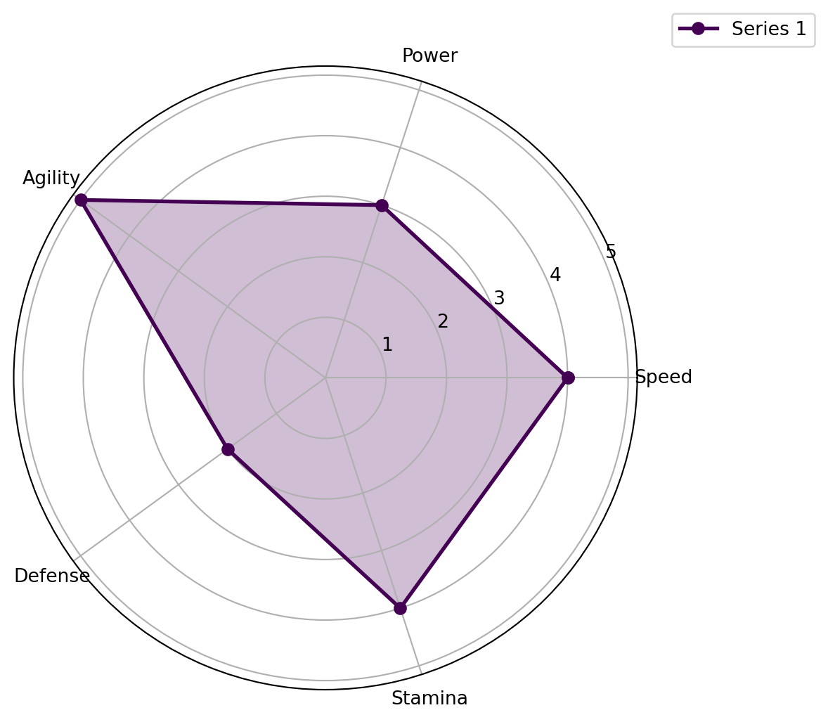
Create a radar (spider) chart.
Excel Usage
=RADAR(data, title, color_map, fill, alpha, legend)data(list[list], required): Input data (Labels, Val1, Val2…).title(str, optional, default: null): Chart title.color_map(str, optional, default: “viridis”): Color map for series.fill(str, optional, default: “true”): Fill the area.alpha(float, optional, default: 0.25): Transparency.legend(str, optional, default: “true”): Show legend.
Returns (object): Matplotlib Figure object (standard Python) or base64 encoded PNG string (Pyodide).
Example 1: Basic radar chart with one series
Inputs:
| data | |
|---|---|
| Speed | 4 |
| Power | 3 |
| Agility | 5 |
| Defense | 2 |
| Stamina | 4 |
Excel formula:
=RADAR({"Speed",4;"Power",3;"Agility",5;"Defense",2;"Stamina",4})Expected output:
"chart"
Example 2: Radar chart with multiple series
Inputs:
| data | ||
|---|---|---|
| A | 3 | 4 |
| B | 4 | 3 |
| C | 5 | 2 |
| D | 2 | 5 |
| E | 4 | 4 |
Excel formula:
=RADAR({"A",3,4;"B",4,3;"C",5,2;"D",2,5;"E",4,4})Expected output:
"chart"
Example 3: Radar chart without fill
Inputs:
| data | fill | |
|---|---|---|
| X | 2 | false |
| Y | 4 | |
| Z | 3 | |
| W | 5 |
Excel formula:
=RADAR({"X",2;"Y",4;"Z",3;"W",5}, "false")Expected output:
"chart"
Example 4: Radar chart with title and legend
Inputs:
| data | title | legend | ||
|---|---|---|---|---|
| Cat1 | 3 | 5 | Comparison | true |
| Cat2 | 4 | 2 | ||
| Cat3 | 5 | 4 |
Excel formula:
=RADAR({"Cat1",3,5;"Cat2",4,2;"Cat3",5,4}, "Comparison", "true")Expected output:
"chart"
Python Code
Show Code
import sys
import matplotlib
IS_PYODIDE = sys.platform == "emscripten"
if IS_PYODIDE:
    matplotlib.use('Agg')
import matplotlib.pyplot as plt
import io
import base64
import numpy as np

def radar(data, title=None, color_map='viridis', fill='true', alpha=0.25, legend='true'):
    """
    Create a radar (spider) chart.

    See: https://matplotlib.org/stable/gallery/specialty_plots/radar_chart.html

    This example function is provided as-is without any representation of accuracy.

    Args:
        data (list[list]): Input data (Labels, Val1, Val2...).
        title (str, optional): Chart title. Default is None.
        color_map (str, optional): Color map for series. Valid options: Viridis, Plasma, Inferno, Magma, Cividis. Default is 'viridis'.
        fill (str, optional): Fill the area. Valid options: True, False. Default is 'true'.
        alpha (float, optional): Transparency. Default is 0.25.
        legend (str, optional): Show legend. Valid options: True, False. Default is 'true'.

    Returns:
        object: Matplotlib Figure object (standard Python) or base64 encoded PNG string (Pyodide).
    """
    def to2d(x):
        return [[x]] if not isinstance(x, list) else x

    try:
        data = to2d(data)

        if not isinstance(data, list) or not all(isinstance(row, list) for row in data):
            return "Error: Invalid input - data must be a 2D list"

        # Transpose data: first column is labels, rest are series
        if len(data) < 1 or len(data[0]) < 2:
            return "Error: Data must have at least 2 columns (Labels, Values)"

        # Extract labels and values
        labels = []
        series = []
        num_series = len(data[0]) - 1

        for _ in range(num_series):
            series.append([])

        for row in data:
            if len(row) >= 2:
                # First column is label
                labels.append(str(row[0]))
                # Remaining columns are values for each series
                for i in range(num_series):
                    if i + 1 < len(row):
                        try:
                            series[i].append(float(row[i + 1]))
                        except (TypeError, ValueError):
                            series[i].append(0)
                    else:
                        series[i].append(0)

        if len(labels) == 0:
            return "Error: No valid data found"

        # Number of variables
        num_vars = len(labels)

        # Compute angle for each axis
        angles = np.linspace(0, 2 * np.pi, num_vars, endpoint=False).tolist()

        # Complete the circle
        angles += angles[:1]

        # Create radar plot
        fig = plt.figure(figsize=(8, 6))
        ax = fig.add_subplot(111, projection='polar')

        # Get colors from colormap
        cmap = plt.get_cmap(color_map)
        colors = cmap(np.linspace(0, 1, num_series))

        # Plot each series
        for i, values in enumerate(series):
            values_plot = values + values[:1]  # Complete the circle
            if fill == "true":
                ax.plot(angles, values_plot, 'o-', linewidth=2, color=colors[i], label=f"Series {i+1}")
                ax.fill(angles, values_plot, alpha=alpha, color=colors[i])
            else:
                ax.plot(angles, values_plot, 'o-', linewidth=2, color=colors[i], label=f"Series {i+1}")

        # Fix axis to go in the right order
        ax.set_xticks(angles[:-1])
        ax.set_xticklabels(labels)

        if title:
            ax.set_title(title)

        if legend == "true":
            ax.legend(loc='upper right', bbox_to_anchor=(1.3, 1.1))

        if IS_PYODIDE:
            buf = io.BytesIO()
            plt.savefig(buf, format='png', bbox_inches='tight')
            plt.close(fig)
            buf.seek(0)
            img_base64 = base64.b64encode(buf.read()).decode('utf-8')
            return f"data:image/png;base64,{img_base64}"
        else:
            return fig
    except Exception as e:
        return f"Error: {str(e)}"
Online Calculator
Input data (Labels, Val1, Val2...).
Chart title.
Color map for series.
Fill the area.
Transparency.
Show legend.
SEMILOGX
Create a plot with a log-scale X-axis.
Excel Usage
=SEMILOGX(data, title, xlabel, ylabel, plot_color, linestyle, marker, legend)data(list[list], required): Input data.title(str, optional, default: null): Chart title.xlabel(str, optional, default: null): Label for X-axis.ylabel(str, optional, default: null): Label for Y-axis.plot_color(str, optional, default: null): Line color.linestyle(str, optional, default: “-”): Line style.marker(str, optional, default: null): Marker style.legend(str, optional, default: “false”): Show legend.
Returns (object): Matplotlib Figure object (standard Python) or base64 encoded PNG string (Pyodide).
Example 1: Basic semi-log X plot
Inputs:
| data | |
|---|---|
| 1 | 2 |
| 10 | 4 |
| 100 | 6 |
| 1000 | 8 |
Excel formula:
=SEMILOGX({1,2;10,4;100,6;1000,8})Expected output:
"chart"
Example 2: Semi-log X with multiple series
Inputs:
| data | legend | ||
|---|---|---|---|
| 1 | 1 | 2 | true |
| 10 | 3 | 4 | |
| 100 | 5 | 6 |
Excel formula:
=SEMILOGX({1,1,2;10,3,4;100,5,6}, "true")Expected output:
"chart"
Example 3: Semi-log X with markers and dashed line
Inputs:
| data | marker | linestyle | |
|---|---|---|---|
| 1 | 1 | s | – |
| 10 | 2 | ||
| 100 | 3 | ||
| 1000 | 4 |
Excel formula:
=SEMILOGX({1,1;10,2;100,3;1000,4}, "s", "--")Expected output:
"chart"
Example 4: Semi-log X with labels and title
Inputs:
| data | title | xlabel | ylabel | |
|---|---|---|---|---|
| 1 | 10 | Semi-log X | X (log) | Y |
| 10 | 20 | |||
| 100 | 30 | |||
| 1000 | 40 |
Excel formula:
=SEMILOGX({1,10;10,20;100,30;1000,40}, "Semi-log X", "X (log)", "Y")Expected output:
"chart"
Python Code
Show Code
import sys
import matplotlib
IS_PYODIDE = sys.platform == "emscripten"
if IS_PYODIDE:
    matplotlib.use('Agg')
import matplotlib.pyplot as plt
import io
import base64
import numpy as np

def semilogx(data, title=None, xlabel=None, ylabel=None, plot_color=None, linestyle='-', marker=None, legend='false'):
    """
    Create a plot with a log-scale X-axis.

    See: https://matplotlib.org/stable/api/_as_gen/matplotlib.pyplot.semilogx.html

    This example function is provided as-is without any representation of accuracy.

    Args:
        data (list[list]): Input data.
        title (str, optional): Chart title. Default is None.
        xlabel (str, optional): Label for X-axis. Default is None.
        ylabel (str, optional): Label for Y-axis. Default is None.
        plot_color (str, optional): Line color. Valid options: Blue, Green, Red, Cyan, Magenta, Yellow, Black, White. Default is None.
        linestyle (str, optional): Line style. Valid options: Solid, Dashed, Dotted, Dash-dot. Default is '-'.
        marker (str, optional): Marker style. Valid options: None, Point, Pixel, Circle, Square, Triangle Down, Triangle Up. Default is None.
        legend (str, optional): Show legend. Valid options: True, False. Default is 'false'.

    Returns:
        object: Matplotlib Figure object (standard Python) or base64 encoded PNG string (Pyodide).
    """
    def to2d(x):
        return [[x]] if not isinstance(x, list) else x

    try:
        data = to2d(data)

        if not isinstance(data, list) or not all(isinstance(row, list) for row in data):
            return "Error: Invalid input - data must be a 2D list"

        # Extract X and Y columns
        if len(data) < 1 or len(data[0]) < 2:
            return "Error: Data must have at least 2 columns"

        # Determine number of series (first column is X, rest are Y series)
        num_series = len(data[0]) - 1

        X = []
        Y_series = [[] for _ in range(num_series)]

        for row in data:
            if len(row) >= 2:
                try:
                    x_val = float(row[0])
                    if x_val > 0:  # Log scale requires positive values
                        X.append(x_val)
                        for i in range(num_series):
                            if i + 1 < len(row):
                                try:
                                    Y_series[i].append(float(row[i + 1]))
                                except (TypeError, ValueError):
                                    Y_series[i].append(None)
                            else:
                                Y_series[i].append(None)
                except (TypeError, ValueError):
                    continue

        if len(X) == 0:
            return "Error: No valid positive X values found"

        # Create semilogx plot
        fig, ax = plt.subplots(figsize=(8, 6))

        # Plot each series
        for i, Y in enumerate(Y_series):
            plot_kwargs = {'linestyle': linestyle}
            if plot_color:
                plot_kwargs['color'] = plot_color
            if marker:
                plot_kwargs['marker'] = marker

            # Filter out None values
            X_filtered = [X[j] for j in range(len(X)) if j < len(Y) and Y[j] is not None]
            Y_filtered = [y for y in Y if y is not None]

            if len(X_filtered) > 0:
                ax.semilogx(X_filtered, Y_filtered, label=f"Series {i+1}", **plot_kwargs)

        if title:
            ax.set_title(title)
        if xlabel:
            ax.set_xlabel(xlabel)
        if ylabel:
            ax.set_ylabel(ylabel)

        if legend == "true" and num_series > 1:
            ax.legend()

        ax.grid(True, which="both", ls="-", alpha=0.2)

        if IS_PYODIDE:
            buf = io.BytesIO()
            plt.savefig(buf, format='png', bbox_inches='tight')
            plt.close(fig)
            buf.seek(0)
            img_base64 = base64.b64encode(buf.read()).decode('utf-8')
            return f"data:image/png;base64,{img_base64}"
        else:
            return fig
    except Exception as e:
        return f"Error: {str(e)}"
Online Calculator
Input data.
Chart title.
Label for X-axis.
Label for Y-axis.
Line color.
Line style.
Marker style.
Show legend.
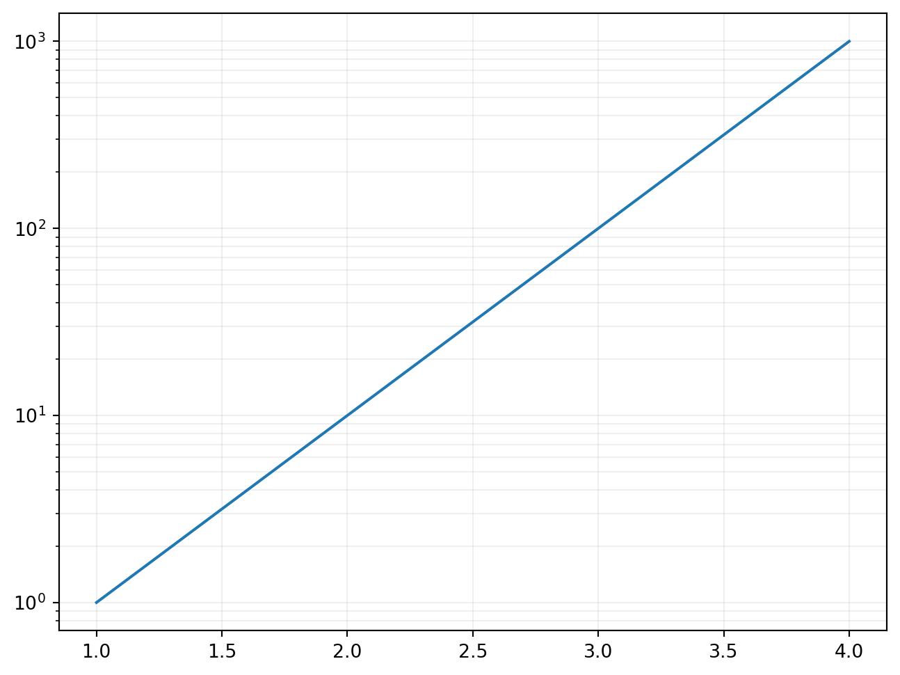
SEMILOGY
Create a plot with a log-scale Y-axis.
Excel Usage
=SEMILOGY(data, title, xlabel, ylabel, plot_color, linestyle, marker, legend)data(list[list], required): Input data.title(str, optional, default: null): Chart title.xlabel(str, optional, default: null): Label for X-axis.ylabel(str, optional, default: null): Label for Y-axis.plot_color(str, optional, default: null): Line color.linestyle(str, optional, default: “-”): Line style.marker(str, optional, default: null): Marker style.legend(str, optional, default: “false”): Show legend.
Returns (object): Matplotlib Figure object (standard Python) or base64 encoded PNG string (Pyodide).
Example 1: Basic semi-log Y plot
Inputs:
| data | |
|---|---|
| 1 | 1 |
| 2 | 10 |
| 3 | 100 |
| 4 | 1000 |
Excel formula:
=SEMILOGY({1,1;2,10;3,100;4,1000})Expected output:
"chart"
Example 2: Semi-log Y with multiple series
Inputs:
| data | legend | ||
|---|---|---|---|
| 1 | 1 | 2 | true |
| 2 | 10 | 20 | |
| 3 | 100 | 200 |
Excel formula:
=SEMILOGY({1,1,2;2,10,20;3,100,200}, "true")Expected output:
"chart"
Example 3: Semi-log Y with markers and color
Inputs:
| data | plot_color | marker | |
|---|---|---|---|
| 0 | 1 | green | ^ |
| 1 | 10 | ||
| 2 | 100 | ||
| 3 | 1000 |
Excel formula:
=SEMILOGY({0,1;1,10;2,100;3,1000}, "green", "^")Expected output:
"chart"
Example 4: Semi-log Y with labels and title
Inputs:
| data | title | xlabel | ylabel | |
|---|---|---|---|---|
| 1 | 1 | Semi-log Y | X | Y (log) |
| 2 | 10 | |||
| 3 | 100 | |||
| 4 | 1000 |
Excel formula:
=SEMILOGY({1,1;2,10;3,100;4,1000}, "Semi-log Y", "X", "Y (log)")Expected output:
"chart"
Python Code
Show Code
import sys
import matplotlib
IS_PYODIDE = sys.platform == "emscripten"
if IS_PYODIDE:
    matplotlib.use('Agg')
import matplotlib.pyplot as plt
import io
import base64
import numpy as np

def semilogy(data, title=None, xlabel=None, ylabel=None, plot_color=None, linestyle='-', marker=None, legend='false'):
    """
    Create a plot with a log-scale Y-axis.

    See: https://matplotlib.org/stable/api/_as_gen/matplotlib.pyplot.semilogy.html

    This example function is provided as-is without any representation of accuracy.

    Args:
        data (list[list]): Input data.
        title (str, optional): Chart title. Default is None.
        xlabel (str, optional): Label for X-axis. Default is None.
        ylabel (str, optional): Label for Y-axis. Default is None.
        plot_color (str, optional): Line color. Valid options: Blue, Green, Red, Cyan, Magenta, Yellow, Black, White. Default is None.
        linestyle (str, optional): Line style. Valid options: Solid, Dashed, Dotted, Dash-dot. Default is '-'.
        marker (str, optional): Marker style. Valid options: None, Point, Pixel, Circle, Square, Triangle Down, Triangle Up. Default is None.
        legend (str, optional): Show legend. Valid options: True, False. Default is 'false'.

    Returns:
        object: Matplotlib Figure object (standard Python) or base64 encoded PNG string (Pyodide).
    """
    def to2d(x):
        return [[x]] if not isinstance(x, list) else x

    try:
        data = to2d(data)

        if not isinstance(data, list) or not all(isinstance(row, list) for row in data):
            return "Error: Invalid input - data must be a 2D list"

        # Extract X and Y columns
        if len(data) < 1 or len(data[0]) < 2:
            return "Error: Data must have at least 2 columns"

        # Determine number of series (first column is X, rest are Y series)
        num_series = len(data[0]) - 1

        X = []
        Y_series = [[] for _ in range(num_series)]

        for row in data:
            if len(row) >= 2:
                try:
                    x_val = float(row[0])
                    X.append(x_val)
                    for i in range(num_series):
                        if i + 1 < len(row):
                            try:
                                y_val = float(row[i + 1])
                                if y_val > 0:  # Log scale requires positive values
                                    Y_series[i].append(y_val)
                                else:
                                    Y_series[i].append(None)
                            except (TypeError, ValueError):
                                Y_series[i].append(None)
                        else:
                            Y_series[i].append(None)
                except (TypeError, ValueError):
                    continue

        if len(X) == 0:
            return "Error: No valid X values found"

        # Check if we have any valid Y values
        has_valid_y = any(any(y is not None for y in Y) for Y in Y_series)
        if not has_valid_y:
            return "Error: No valid positive Y values found"

        # Create semilogy plot
        fig, ax = plt.subplots(figsize=(8, 6))

        # Plot each series
        for i, Y in enumerate(Y_series):
            plot_kwargs = {'linestyle': linestyle}
            if plot_color:
                plot_kwargs['color'] = plot_color
            if marker:
                plot_kwargs['marker'] = marker

            # Filter out None values
            X_filtered = [X[j] for j in range(len(X)) if j < len(Y) and Y[j] is not None]
            Y_filtered = [y for y in Y if y is not None]

            if len(X_filtered) > 0:
                ax.semilogy(X_filtered, Y_filtered, label=f"Series {i+1}", **plot_kwargs)

        if title:
            ax.set_title(title)
        if xlabel:
            ax.set_xlabel(xlabel)
        if ylabel:
            ax.set_ylabel(ylabel)

        if legend == "true" and num_series > 1:
            ax.legend()

        ax.grid(True, which="both", ls="-", alpha=0.2)

        if IS_PYODIDE:
            buf = io.BytesIO()
            plt.savefig(buf, format='png', bbox_inches='tight')
            plt.close(fig)
            buf.seek(0)
            img_base64 = base64.b64encode(buf.read()).decode('utf-8')
            return f"data:image/png;base64,{img_base64}"
        else:
            return fig
    except Exception as e:
        return f"Error: {str(e)}"
Online Calculator
Input data.
Chart title.
Label for X-axis.
Label for Y-axis.
Line color.
Line style.
Marker style.
Show legend.
STREAMPLOT
Create a streamplot (vector field streamlines).
Excel Usage
=STREAMPLOT(data, title, xlabel, ylabel, color_map, density)data(list[list], required): Input data (X, Y, U, V).title(str, optional, default: null): Chart title.xlabel(str, optional, default: null): Label for X-axis.ylabel(str, optional, default: null): Label for Y-axis.color_map(str, optional, default: “viridis”): Color map for streamlines.density(float, optional, default: 1): Density of streamlines.
Returns (object): Matplotlib Figure object (standard Python) or base64 encoded PNG string (Pyodide).
Example 1: Basic streamplot
Inputs:
| data | |||
|---|---|---|---|
| 0 | 0 | 1 | 0 |
| 1 | 0 | 1 | 0 |
| 0 | 1 | 1 | 1 |
| 1 | 1 | 1 | 1 |
Excel formula:
=STREAMPLOT({0,0,1,0;1,0,1,0;0,1,1,1;1,1,1,1})Expected output:
"chart"
Example 2: Streamplot with plasma colormap
Inputs:
| data | color_map | |||
|---|---|---|---|---|
| 0 | 0 | 1 | 0 | plasma |
| 1 | 0 | 0 | 1 | |
| 2 | 0 | -1 | 0 | |
| 0 | 1 | 1 | 1 | |
| 1 | 1 | 0 | 0 | |
| 2 | 1 | -1 | 1 |
Excel formula:
=STREAMPLOT({0,0,1,0;1,0,0,1;2,0,-1,0;0,1,1,1;1,1,0,0;2,1,-1,1}, "plasma")Expected output:
"chart"
Example 3: Streamplot with labels and title
Inputs:
| data | title | xlabel | ylabel | |||
|---|---|---|---|---|---|---|
| 0 | 0 | 1 | 1 | Flow Field | X | Y |
| 1 | 0 | -1 | 1 | |||
| 0 | 1 | 1 | -1 | |||
| 1 | 1 | -1 | -1 |
Excel formula:
=STREAMPLOT({0,0,1,1;1,0,-1,1;0,1,1,-1;1,1,-1,-1}, "Flow Field", "X", "Y")Expected output:
"chart"
Example 4: Streamplot with higher density
Inputs:
| data | density | |||
|---|---|---|---|---|
| 0 | 0 | 1 | 0 | 2 |
| 1 | 0 | 0 | 1 | |
| 0 | 1 | -1 | 0 | |
| 1 | 1 | 0 | -1 |
Excel formula:
=STREAMPLOT({0,0,1,0;1,0,0,1;0,1,-1,0;1,1,0,-1}, 2)Expected output:
"chart"
Python Code
Show Code
import sys
import matplotlib
IS_PYODIDE = sys.platform == "emscripten"
if IS_PYODIDE:
    matplotlib.use('Agg')
import matplotlib.pyplot as plt
import io
import base64
import numpy as np

def streamplot(data, title=None, xlabel=None, ylabel=None, color_map='viridis', density=1):
    """
    Create a streamplot (vector field streamlines).

    See: https://matplotlib.org/stable/api/_as_gen/matplotlib.pyplot.streamplot.html

    This example function is provided as-is without any representation of accuracy.

    Args:
        data (list[list]): Input data (X, Y, U, V).
        title (str, optional): Chart title. Default is None.
        xlabel (str, optional): Label for X-axis. Default is None.
        ylabel (str, optional): Label for Y-axis. Default is None.
        color_map (str, optional): Color map for streamlines. Valid options: Viridis, Plasma, Inferno, Magma, Cividis. Default is 'viridis'.
        density (float, optional): Density of streamlines. Default is 1.

    Returns:
        object: Matplotlib Figure object (standard Python) or base64 encoded PNG string (Pyodide).
    """
    def to2d(x):
        return [[x]] if not isinstance(x, list) else x

    try:
        data = to2d(data)

        if not isinstance(data, list) or not all(isinstance(row, list) for row in data):
            return "Error: Invalid input - data must be a 2D list"

        # Extract X, Y, U, V columns
        if len(data) < 1 or len(data[0]) < 4:
            return "Error: Data must have at least 4 columns (X, Y, U, V)"

        X = []
        Y = []
        U = []
        V = []
        for row in data:
            if len(row) >= 4:
                try:
                    X.append(float(row[0]))
                    Y.append(float(row[1]))
                    U.append(float(row[2]))
                    V.append(float(row[3]))
                except (TypeError, ValueError):
                    continue

        if len(X) == 0:
            return "Error: No valid numeric data found"

        # Convert to unique grid points
        X_unique = sorted(list(set(X)))
        Y_unique = sorted(list(set(Y)))

        if len(X_unique) < 2 or len(Y_unique) < 2:
            return "Error: Need at least 2 unique X and Y values for streamplot"

        # Create meshgrid
        X_grid, Y_grid = np.meshgrid(X_unique, Y_unique)

        # Interpolate U and V onto grid
        U_grid = np.zeros_like(X_grid)
        V_grid = np.zeros_like(Y_grid)

        for i in range(len(X)):
            xi = X_unique.index(X[i])
            yi = Y_unique.index(Y[i])
            U_grid[yi, xi] = U[i]
            V_grid[yi, xi] = V[i]

        # Create streamplot
        fig, ax = plt.subplots(figsize=(8, 6))

        strm = ax.streamplot(X_grid, Y_grid, U_grid, V_grid, color=np.sqrt(U_grid**2 + V_grid**2),
                             cmap=color_map, density=density)

        if title:
            ax.set_title(title)
        if xlabel:
            ax.set_xlabel(xlabel)
        if ylabel:
            ax.set_ylabel(ylabel)

        if IS_PYODIDE:
            buf = io.BytesIO()
            plt.savefig(buf, format='png', bbox_inches='tight')
            plt.close(fig)
            buf.seek(0)
            img_base64 = base64.b64encode(buf.read()).decode('utf-8')
            return f"data:image/png;base64,{img_base64}"
        else:
            return fig
    except Exception as e:
        return f"Error: {str(e)}"
Online Calculator
Input data (X, Y, U, V).
Chart title.
Label for X-axis.
Label for Y-axis.
Color map for streamlines.
Density of streamlines.
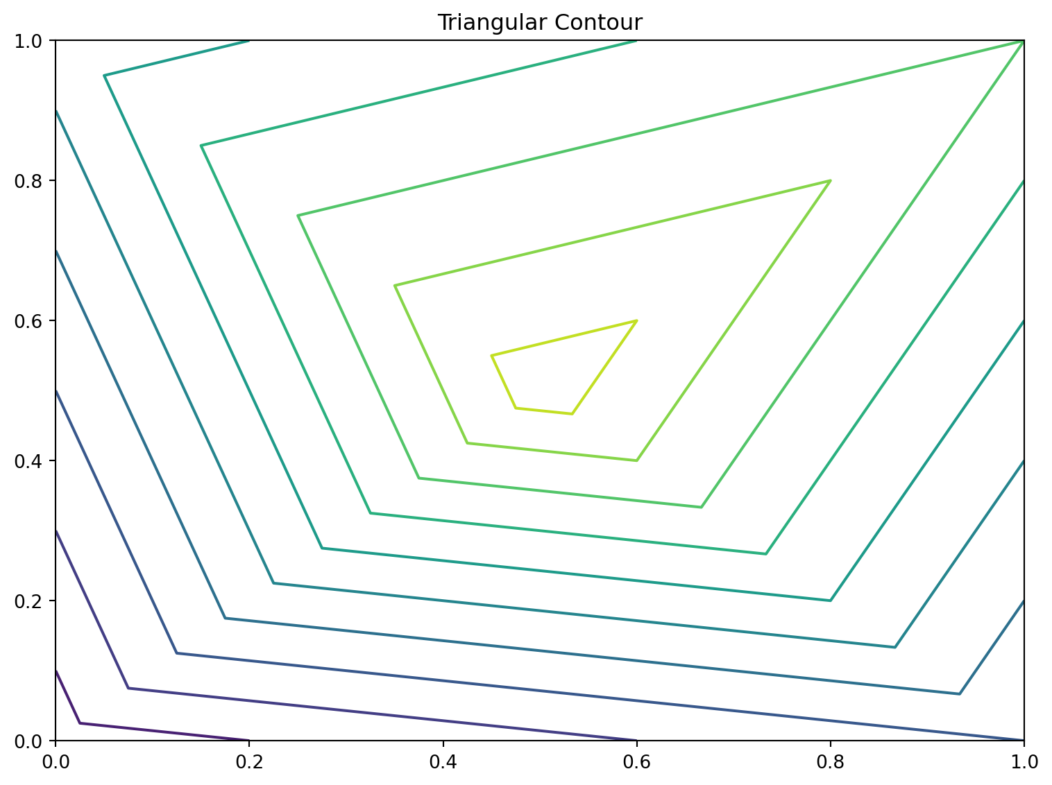
TRICONTOUR
Draw contour lines on an unstructured triangular grid.
Excel Usage
=TRICONTOUR(data, title, xlabel, ylabel, color_map, levels)data(list[list], required): Input data with 3 columns (X, Y, Z).title(str, optional, default: null): Chart title.xlabel(str, optional, default: null): Label for X-axis.ylabel(str, optional, default: null): Label for Y-axis.color_map(str, optional, default: “viridis”): Color map for contours.levels(int, optional, default: 10): Number of contour levels.
Returns (object): Matplotlib Figure object (standard Python) or base64 encoded PNG string (Pyodide).
Example 1: Simple unstructured contour
Inputs:
| data | title | ||
|---|---|---|---|
| 0 | 0 | 1 | Triangular Contour |
| 1 | 0 | 2 | |
| 0 | 1 | 3 | |
| 1 | 1 | 4 | |
| 0.5 | 0.5 | 5 |
Excel formula:
=TRICONTOUR({0,0,1;1,0,2;0,1,3;1,1,4;0.5,0.5,5}, "Triangular Contour")Expected output:
"chart"
Example 2: Contour with inferno map
Inputs:
| data | color_map | ||
|---|---|---|---|
| 0 | 0 | 1 | inferno |
| 2 | 0 | 10 | |
| 1 | 2 | 5 |
Excel formula:
=TRICONTOUR({0,0,1;2,0,10;1,2,5}, "inferno")Expected output:
"chart"
Example 3: Contour with 20 levels
Inputs:
| data | levels | ||
|---|---|---|---|
| 0 | 0 | 1 | 20 |
| 5 | 0 | 2 | |
| 2 | 5 | 3 |
Excel formula:
=TRICONTOUR({0,0,1;5,0,2;2,5,3}, 20)Expected output:
"chart"
Example 4: Contour with plasma map
Inputs:
| data | color_map | ||
|---|---|---|---|
| 0 | 0 | 1 | plasma |
| 1 | 1 | 10 | |
| 2 | 0 | 5 |
Excel formula:
=TRICONTOUR({0,0,1;1,1,10;2,0,5}, "plasma")Expected output:
"chart"
Python Code
Show Code
import sys
import matplotlib
IS_PYODIDE = sys.platform == "emscripten"
if IS_PYODIDE:
    matplotlib.use('Agg')
import matplotlib.pyplot as plt
import io
import base64
import numpy as np

def tricontour(data, title=None, xlabel=None, ylabel=None, color_map='viridis', levels=10):
    """
    Draw contour lines on an unstructured triangular grid.

    See: https://matplotlib.org/stable/api/_as_gen/matplotlib.pyplot.tricontour.html

    This example function is provided as-is without any representation of accuracy.

    Args:
        data (list[list]): Input data with 3 columns (X, Y, Z).
        title (str, optional): Chart title. Default is None.
        xlabel (str, optional): Label for X-axis. Default is None.
        ylabel (str, optional): Label for Y-axis. Default is None.
        color_map (str, optional): Color map for contours. Valid options: Viridis, Plasma, Inferno, Magma, Cividis. Default is 'viridis'.
        levels (int, optional): Number of contour levels. Default is 10.

    Returns:
        object: Matplotlib Figure object (standard Python) or base64 encoded PNG string (Pyodide).
    """
    def to2d(x):
        return [[x]] if not isinstance(x, list) else x

    try:
        data = to2d(data)
        if not isinstance(data, list) or not data or not isinstance(data[0], list):
            return "Error: Input data must be a 2D list."

        # Convert to numpy array
        try:
            arr = np.array(data, dtype=float)
        except Exception:
            return "Error: Data must be numeric."

        if arr.shape[1] < 3:
            return "Error: Data must have at least 3 columns (X, Y, Z)."

        # Extract coordinates
        x, y, z = arr[:, 0], arr[:, 1], arr[:, 2]

        # Create figure
        fig, ax = plt.subplots(figsize=(8, 6))

        # Plot tricontour
        ax.tricontour(x, y, z, levels=levels, cmap=color_map)

        # Set labels and title
        if title:
            ax.set_title(title)
        if xlabel:
            ax.set_xlabel(xlabel)
        if ylabel:
            ax.set_ylabel(ylabel)

        plt.tight_layout()

        if IS_PYODIDE:
            buf = io.BytesIO()
            plt.savefig(buf, format='png', dpi=100, bbox_inches='tight')
            plt.close(fig)
            buf.seek(0)
            img_bytes = buf.read()
            img_b64 = base64.b64encode(img_bytes).decode('utf-8')
            return f"data:image/png;base64,{img_b64}"
        else:
            return fig
    except Exception as e:
        return f"Error: {str(e)}"
Online Calculator
Input data with 3 columns (X, Y, Z).
Chart title.
Label for X-axis.
Label for Y-axis.
Color map for contours.
Number of contour levels.
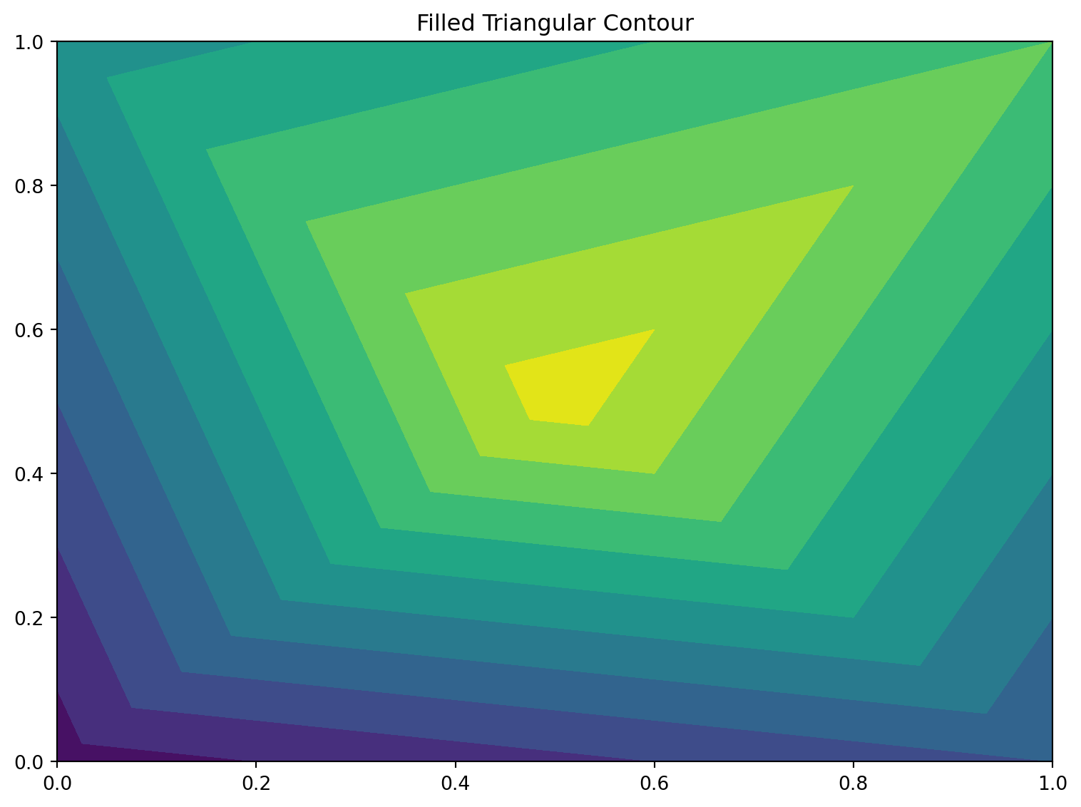
TRICONTOUR_FILLED
Draw filled contour regions on an unstructured triangular grid.
Excel Usage
=TRICONTOUR_FILLED(data, title, xlabel, ylabel, color_map, levels)data(list[list], required): Input data with 3 columns (X, Y, Z).title(str, optional, default: null): Chart title.xlabel(str, optional, default: null): Label for X-axis.ylabel(str, optional, default: null): Label for Y-axis.color_map(str, optional, default: “viridis”): Color map for regions.levels(int, optional, default: 10): Number of contour levels.
Returns (object): Matplotlib Figure object (standard Python) or base64 encoded PNG string (Pyodide).
Example 1: Simple filled unstructured contour
Inputs:
| data | title | ||
|---|---|---|---|
| 0 | 0 | 1 | Filled Triangular Contour |
| 1 | 0 | 2 | |
| 0 | 1 | 3 | |
| 1 | 1 | 4 | |
| 0.5 | 0.5 | 5 |
Excel formula:
=TRICONTOUR_FILLED({0,0,1;1,0,2;0,1,3;1,1,4;0.5,0.5,5}, "Filled Triangular Contour")Expected output:
"chart"
Example 2: Filled contour with plasma map
Inputs:
| data | color_map | ||
|---|---|---|---|
| 0 | 0 | 1 | plasma |
| 2 | 0 | 10 | |
| 1 | 2 | 5 |
Excel formula:
=TRICONTOUR_FILLED({0,0,1;2,0,10;1,2,5}, "plasma")Expected output:
"chart"
Example 3: High resolution triangular filled
Inputs:
| data | levels | ||
|---|---|---|---|
| 0 | 0 | 0 | 15 |
| 1 | 0 | 1 | |
| 0.5 | 0.866 | 2 | |
| 0.5 | 0.288 | 5 |
Excel formula:
=TRICONTOUR_FILLED({0,0,0;1,0,1;0.5,0.866,2;0.5,0.288,5}, 15)Expected output:
"chart"
Example 4: Filled contour with magma map
Inputs:
| data | color_map | ||
|---|---|---|---|
| 0 | 0 | 1 | magma |
| 1 | 0 | 2 | |
| 0 | 1 | 3 | |
| 1 | 1 | 4 |
Excel formula:
=TRICONTOUR_FILLED({0,0,1;1,0,2;0,1,3;1,1,4}, "magma")Expected output:
"chart"
Python Code
Show Code
import sys
import matplotlib
IS_PYODIDE = sys.platform == "emscripten"
if IS_PYODIDE:
    matplotlib.use('Agg')
import matplotlib.pyplot as plt
import io
import base64
import numpy as np

def tricontour_filled(data, title=None, xlabel=None, ylabel=None, color_map='viridis', levels=10):
    """
    Draw filled contour regions on an unstructured triangular grid.

    See: https://matplotlib.org/stable/api/_as_gen/matplotlib.pyplot.tricontourf.html

    This example function is provided as-is without any representation of accuracy.

    Args:
        data (list[list]): Input data with 3 columns (X, Y, Z).
        title (str, optional): Chart title. Default is None.
        xlabel (str, optional): Label for X-axis. Default is None.
        ylabel (str, optional): Label for Y-axis. Default is None.
        color_map (str, optional): Color map for regions. Valid options: Viridis, Plasma, Inferno, Magma, Cividis. Default is 'viridis'.
        levels (int, optional): Number of contour levels. Default is 10.

    Returns:
        object: Matplotlib Figure object (standard Python) or base64 encoded PNG string (Pyodide).
    """
    def to2d(x):
        return [[x]] if not isinstance(x, list) else x

    try:
        data = to2d(data)
        if not isinstance(data, list) or not data or not isinstance(data[0], list):
            return "Error: Input data must be a 2D list."

        # Convert to numpy array
        try:
            arr = np.array(data, dtype=float)
        except Exception:
            return "Error: Data must be numeric."

        if arr.shape[1] < 3:
            return "Error: Data must have at least 3 columns (X, Y, Z)."

        # Extract coordinates
        x, y, z = arr[:, 0], arr[:, 1], arr[:, 2]

        # Create figure
        fig, ax = plt.subplots(figsize=(8, 6))

        # Plot filled tricontour
        ax.tricontourf(x, y, z, levels=levels, cmap=color_map)

        # Set labels and title
        if title:
            ax.set_title(title)
        if xlabel:
            ax.set_xlabel(xlabel)
        if ylabel:
            ax.set_ylabel(ylabel)

        plt.tight_layout()

        if IS_PYODIDE:
            buf = io.BytesIO()
            plt.savefig(buf, format='png', dpi=100, bbox_inches='tight')
            plt.close(fig)
            buf.seek(0)
            img_bytes = buf.read()
            img_b64 = base64.b64encode(img_bytes).decode('utf-8')
            return f"data:image/png;base64,{img_b64}"
        else:
            return fig
    except Exception as e:
        return f"Error: {str(e)}"
Online Calculator
Input data with 3 columns (X, Y, Z).
Chart title.
Label for X-axis.
Label for Y-axis.
Color map for regions.
Number of contour levels.
TRIPCOLOR
Create a pseudocolor plot of an unstructured triangular grid.
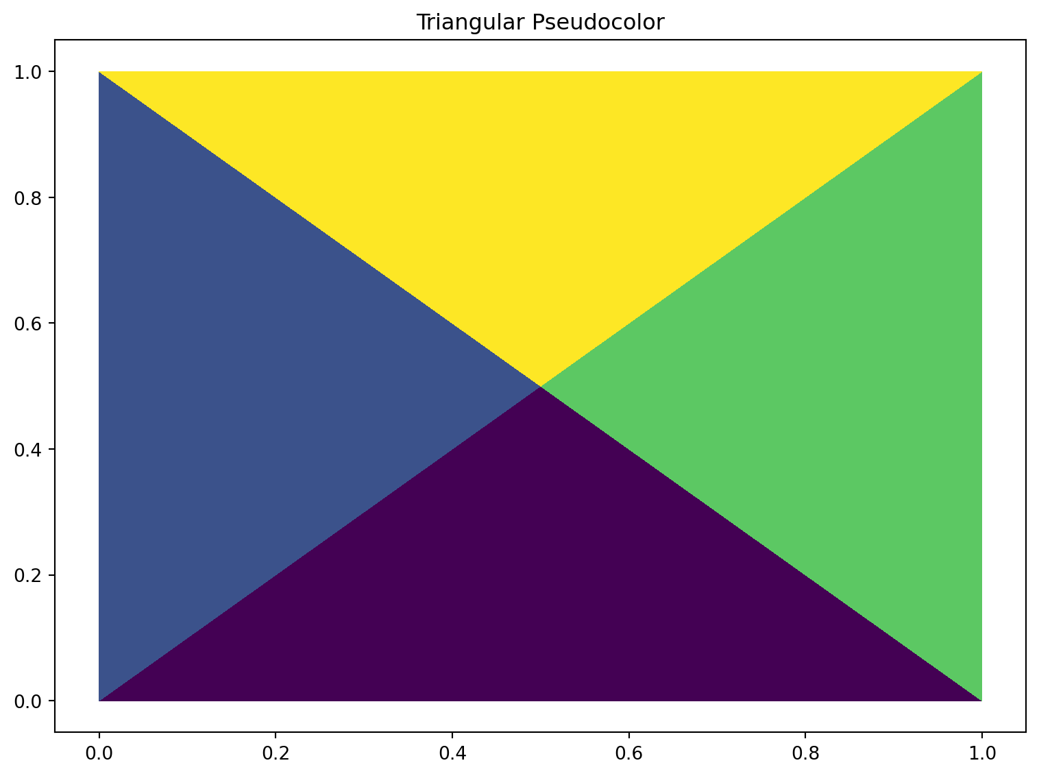
Excel Usage
=TRIPCOLOR(data, title, xlabel, ylabel, color_map)data(list[list], required): Input data with 3 columns (X, Y, Z).title(str, optional, default: null): Chart title.xlabel(str, optional, default: null): Label for X-axis.ylabel(str, optional, default: null): Label for Y-axis.color_map(str, optional, default: “viridis”): Color map for plot.
Returns (object): Matplotlib Figure object (standard Python) or base64 encoded PNG string (Pyodide).
Example 1: Simple triangular pseudocolor
Inputs:
| data | title | ||
|---|---|---|---|
| 0 | 0 | 1 | Triangular Pseudocolor |
| 1 | 0 | 2 | |
| 0 | 1 | 3 | |
| 1 | 1 | 4 | |
| 0.5 | 0.5 | 5 |
Excel formula:
=TRIPCOLOR({0,0,1;1,0,2;0,1,3;1,1,4;0.5,0.5,5}, "Triangular Pseudocolor")Expected output:
"chart"
Example 2: Pseudocolor with magma map
Inputs:
| data | color_map | ||
|---|---|---|---|
| 0 | 0 | 1 | magma |
| 2 | 0 | 10 | |
| 1 | 2 | 5 |
Excel formula:
=TRIPCOLOR({0,0,1;2,0,10;1,2,5}, "magma")Expected output:
"chart"
Example 3: Pseudocolor with cividis map
Inputs:
| data | color_map | ||
|---|---|---|---|
| 0 | 0 | 1 | cividis |
| 1 | 1 | 5 | |
| 2 | 0 | 2 |
Excel formula:
=TRIPCOLOR({0,0,1;1,1,5;2,0,2}, "cividis")Expected output:
"chart"
Example 4: Pseudocolor with inferno map
Inputs:
| data | color_map | ||
|---|---|---|---|
| 0 | 0 | 5 | inferno |
| 1 | 0 | 1 | |
| 0 | 1 | 10 |
Excel formula:
=TRIPCOLOR({0,0,5;1,0,1;0,1,10}, "inferno")Expected output:
"chart"
Python Code
Show Code
import sys
import matplotlib
IS_PYODIDE = sys.platform == "emscripten"
if IS_PYODIDE:
    matplotlib.use('Agg')
import matplotlib.pyplot as plt
import io
import base64
import numpy as np

def tripcolor(data, title=None, xlabel=None, ylabel=None, color_map='viridis'):
    """
    Create a pseudocolor plot of an unstructured triangular grid.

    See: https://matplotlib.org/stable/api/_as_gen/matplotlib.pyplot.tripcolor.html

    This example function is provided as-is without any representation of accuracy.

    Args:
        data (list[list]): Input data with 3 columns (X, Y, Z).
        title (str, optional): Chart title. Default is None.
        xlabel (str, optional): Label for X-axis. Default is None.
        ylabel (str, optional): Label for Y-axis. Default is None.
        color_map (str, optional): Color map for plot. Valid options: Viridis, Plasma, Inferno, Magma, Cividis. Default is 'viridis'.

    Returns:
        object: Matplotlib Figure object (standard Python) or base64 encoded PNG string (Pyodide).
    """
    def to2d(x):
        return [[x]] if not isinstance(x, list) else x

    try:
        data = to2d(data)
        if not isinstance(data, list) or not data or not isinstance(data[0], list):
            return "Error: Input data must be a 2D list."

        # Convert to numpy array
        try:
            arr = np.array(data, dtype=float)
        except Exception:
            return "Error: Data must be numeric."

        if arr.shape[1] < 3:
            return "Error: Data must have at least 3 columns (X, Y, Z)."

        # Extract coordinates
        x, y, z = arr[:, 0], arr[:, 1], arr[:, 2]

        # Create figure
        fig, ax = plt.subplots(figsize=(8, 6))

        # Plot tripcolor
        ax.tripcolor(x, y, z, cmap=color_map)

        # Set labels and title
        if title:
            ax.set_title(title)
        if xlabel:
            ax.set_xlabel(xlabel)
        if ylabel:
            ax.set_ylabel(ylabel)

        plt.tight_layout()

        if IS_PYODIDE:
            buf = io.BytesIO()
            plt.savefig(buf, format='png', dpi=100, bbox_inches='tight')
            plt.close(fig)
            buf.seek(0)
            img_bytes = buf.read()
            img_b64 = base64.b64encode(img_bytes).decode('utf-8')
            return f"data:image/png;base64,{img_b64}"
        else:
            return fig
    except Exception as e:
        return f"Error: {str(e)}"
Online Calculator
Input data with 3 columns (X, Y, Z).
Chart title.
Label for X-axis.
Label for Y-axis.
Color map for plot.
TRIPLOT
Draw an unstructured triangular grid as lines and/or markers.
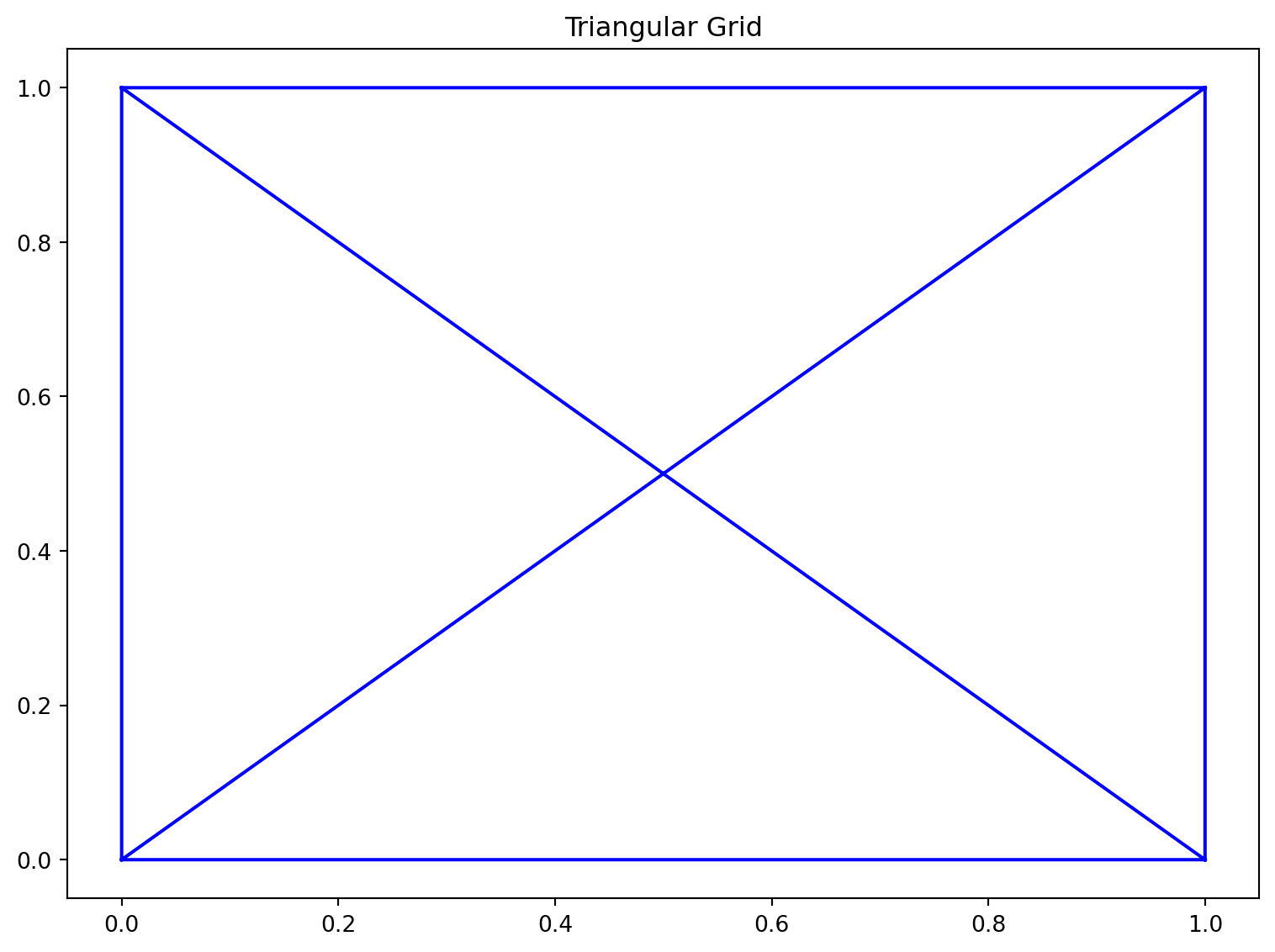
Excel Usage
=TRIPLOT(data, title, xlabel, ylabel, line_color, marker)data(list[list], required): Input data with 2 columns (X, Y).title(str, optional, default: null): Chart title.xlabel(str, optional, default: null): Label for X-axis.ylabel(str, optional, default: null): Label for Y-axis.line_color(str, optional, default: “blue”): Color of the grid lines.marker(str, optional, default: “none”): Marker style for points.
Returns (object): Matplotlib Figure object (standard Python) or base64 encoded PNG string (Pyodide).
Example 1: Simple triangular grid lines
Inputs:
| data | title | |
|---|---|---|
| 0 | 0 | Triangular Grid |
| 1 | 0 | |
| 0 | 1 | |
| 1 | 1 | |
| 0.5 | 0.5 |
Excel formula:
=TRIPLOT({0,0;1,0;0,1;1,1;0.5,0.5}, "Triangular Grid")Expected output:
"chart"
Example 2: Grid lines with markers
Inputs:
| data | marker | line_color | |
|---|---|---|---|
| 0 | 0 | o | red |
| 1 | 0 | ||
| 0.5 | 0.866 |
Excel formula:
=TRIPLOT({0,0;1,0;0.5,0.866}, "o", "red")Expected output:
"chart"
Example 3: Grid lines with square markers
Inputs:
| data | marker | line_color | |
|---|---|---|---|
| 0 | 0 | s | green |
| 2 | 0 | ||
| 1 | 2 |
Excel formula:
=TRIPLOT({0,0;2,0;1,2}, "s", "green")Expected output:
"chart"
Example 4: Simple black grid lines
Inputs:
| data | line_color | |
|---|---|---|
| 0 | 0 | black |
| 1 | 1 | |
| 1 | 0 |
Excel formula:
=TRIPLOT({0,0;1,1;1,0}, "black")Expected output:
"chart"
Python Code
Show Code
import sys
import matplotlib
IS_PYODIDE = sys.platform == "emscripten"
if IS_PYODIDE:
    matplotlib.use('Agg')
import matplotlib.pyplot as plt
import io
import base64
import numpy as np

def triplot(data, title=None, xlabel=None, ylabel=None, line_color='blue', marker='none'):
    """
    Draw an unstructured triangular grid as lines and/or markers.

    See: https://matplotlib.org/stable/api/_as_gen/matplotlib.pyplot.triplot.html

    This example function is provided as-is without any representation of accuracy.

    Args:
        data (list[list]): Input data with 2 columns (X, Y).
        title (str, optional): Chart title. Default is None.
        xlabel (str, optional): Label for X-axis. Default is None.
        ylabel (str, optional): Label for Y-axis. Default is None.
        line_color (str, optional): Color of the grid lines. Valid options: Blue, Green, Red, Black. Default is 'blue'.
        marker (str, optional): Marker style for points. Valid options: None, Point, Pixel, Circle, Square, Triangle Down, Triangle Up. Default is 'none'.

    Returns:
        object: Matplotlib Figure object (standard Python) or base64 encoded PNG string (Pyodide).
    """
    def to2d(x):
        return [[x]] if not isinstance(x, list) else x

    try:
        data = to2d(data)
        if not isinstance(data, list) or not data or not isinstance(data[0], list):
            return "Error: Input data must be a 2D list."

        # Convert to numpy array
        try:
            arr = np.array(data, dtype=float)
        except Exception:
            return "Error: Data must be numeric."

        if arr.shape[1] < 2:
            return "Error: Data must have at least 2 columns (X, Y)."

        # Extract coordinates
        x, y = arr[:, 0], arr[:, 1]

        # Create figure
        fig, ax = plt.subplots(figsize=(8, 6))

        # Plot triplot
        ax.triplot(x, y, color=line_color, marker=marker if marker else None)

        # Set labels and title
        if title:
            ax.set_title(title)
        if xlabel:
            ax.set_xlabel(xlabel)
        if ylabel:
            ax.set_ylabel(ylabel)

        plt.tight_layout()

        if IS_PYODIDE:
            buf = io.BytesIO()
            plt.savefig(buf, format='png', dpi=100, bbox_inches='tight')
            plt.close(fig)
            buf.seek(0)
            img_bytes = buf.read()
            img_b64 = base64.b64encode(img_bytes).decode('utf-8')
            return f"data:image/png;base64,{img_b64}"
        else:
            return fig
    except Exception as e:
        return f"Error: {str(e)}"
Online Calculator
Input data with 2 columns (X, Y).
Chart title.
Label for X-axis.
Label for Y-axis.
Color of the grid lines.
Marker style for points.