Solver for Excel
Overview
The Solver Add-in brings powerful SciPy optimization algorithms directly to Excel as custom functions.

Features
| Feature | Description |
|---|---|
| 🆓 Free | Unlimited free use |
| 🌐 Cross-Platform | Works in Excel for web and desktop |
| ✅ Flexible Runtime | Use Excel =PY() or local Python runtime |
| 🔒 Private | No data is shared outside Excel |
| 🔍 Transparent | Python source code available for review |
How It Works
Use functions directly in Excel cells (e.g., =SOLVER.MINIMIZE(...)) like native functions. All custom functions use the SOLVER. prefix.
Two ways to use functions:
| Method | Description |
|---|---|
| Type directly | Enter formulas like =SOLVER.MINIMIZE("x^2 + y^2", {1, 1}) |
| Function Dialog | Guided experience from the taskpane |
Custom functions use Pyodide in Excel's add-in browser—no Python installation needed.
Key Concept
All functions use mathematical expressions (e.g., x^2 + y^2), to define the objective function.
User Guide
Getting Started
Open the Solver taskpane via the Solver ribbon button. Sign in with your current Excel Microsoft account. Grant permissions on first use. Revoke consent via work accounts or personal accounts.
You can now use the Solver functions in your Excel workbook by typing =SOLVER. and selecting a function from the dropdown. You can also use the Solver taskpane to select a function and enter arguments following a three-step workflow:
- Select Function — Search or browse by category
- Enter Arguments — Fill parameters with live previews
- Insert — Choose formula, static result, or
=PY()formula
Select Function
:::
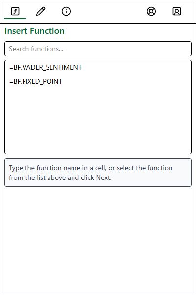
Search by name/keyword or browse by category.
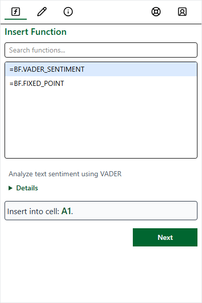
Select a function to see details, then click Next. :::
Enter Arguments
| Method | Description |
|---|---|
| Type directly | Text, numbers, or arrays (e.g., {1,2;3,4}) |
| Select range | Click field, then select cells |
| Use Test Values | Populate with defaults |
:::
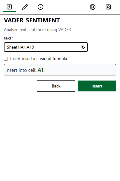
Click field and select cells.
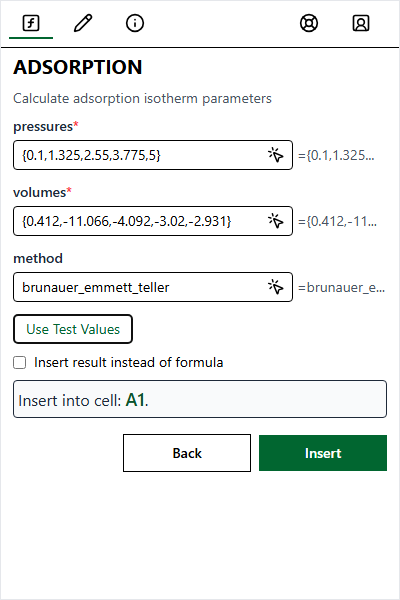
Test values include sample arrays. :::
Insert Options
| Option | Description |
|---|---|
| Formula (default) | Dynamic formula, e.g. =SOLVER.MINIMIZE(...) |
| Result | Static computed value that will not update |
| =PY() formula | Excel's Python environment (selected functions only) |
Errors
| Error | Cause | Solution |
|---|---|---|
#VALUE! | Wrong type or missing argument | Check argument types |
#NAME? | Unrecognized function | Check spelling and SOLVER. prefix |
#BUSY! | Processing (normal on first use) | Wait; if persistent, click Reset |
Functions
14 optimization functions in five categories. Click for full documentation.
Assignment Problems
| Function | Description |
|---|---|
| LINEAR_ASSIGNMENT | Solve linear assignment problem |
| QUADRATIC_ASSIGNMENT | Solve quadratic assignment problem |
Global Optimization
| Function | Description |
|---|---|
| BASIN_HOPPING | Basin-hopping algorithm |
| BRUTE | Brute-force grid search |
| DIFFERENTIAL_EVOLUTION | Differential evolution |
| DUAL_ANNEALING | Dual annealing |
| SHGO | Simplicial Homology Global Optimization |
Linear Programming
| Function | Description |
|---|---|
| LINEAR_PROG | Linear programming |
| MILP | Mixed-integer linear program |
Local Optimization
| Function | Description |
|---|---|
| MINIMIZE | Multivariate minimization |
| MINIMIZE_SCALAR | Single-variable minimization |
Root Finding
| Function | Description |
|---|---|
| FIXED_POINT | Find fixed point f(x) = x |
| ROOT | Solve nonlinear system |
| ROOT_SCALAR | Find scalar root |
Excel Resources
| Tool | Best For | Limitations |
|---|---|---|
| This Add-in | Large/advanced problems, programmatic control | Math expressions only |
| Excel Solver | Small formula-based models (≤200 vars) | Limited algorithms, slower |
| Goal Seek | Single-variable target seeking | One variable only |
| Analysis ToolPak | Basic linear regression | No nonlinear fitting |