Reduction

Overview

Introduction In control engineering, model order reduction is the process of replacing a high-order dynamic model with a lower-order model that preserves the behavior that matters for analysis, design, and simulation. A full-order plant model often comes from first-principles physics, finite-element discretization, or system identification, and can be too large for fast iteration. Reduction methods produce a compact surrogate that runs faster, is easier to interpret, and is often more numerically robust for controller design loops.

Mathematically, model reduction seeks a reduced state-space realization \dot x_r = A_r x_r + B_r u,\quad y_r = C_r x_r + D_r u with order r \ll n such that the input-output behavior approximates the original model \dot x = A x + B u,\quad y = C x + D u. The objective is not merely compression; it is compression with guarantees or practical confidence around stability, low-frequency gain, transient shape, and frequency response over the operating region.

For business and engineering teams, this matters because control decisions are made under time and compute constraints. A digital twin that takes minutes to simulate per scenario can block design-space exploration, Monte Carlo robustness studies, and embedded deployment. A reduced model can cut that runtime by orders of magnitude while retaining the dynamics needed for tuning and validation. In hardware-in-the-loop and model-predictive control, this speed difference directly affects whether the workflow is viable.

Boardflare’s reduction category focuses on two high-impact operations built on the Python Control Systems Library:

• MINREAL: removes mathematically redundant dynamics (uncontrollable/unobservable states or canceling pole-zero factors), yielding a minimal realization with equivalent transfer behavior.
• BALRED: performs balanced truncation-style reduction to intentionally approximate the system with fewer states when exact minimality alone is not enough.

These functions correspond to capabilities in python-control model simplification APIs (notably minimal_realization and balanced_reduction). Conceptually, they sit within the broader model order reduction literature, but they are packaged here for practical, spreadsheet-friendly engineering workflows.

When to Use It Use reduction when the “full” model is correct but operationally inconvenient. The key distinction is whether you need exact simplification (remove only redundancy) or approximate simplification (remove low-impact dynamics intentionally).

A common job-to-be-done is accelerating controller iteration during product development. Suppose a mechatronics team has a 40-state linearized plant from CAD + multibody simulation. Early tuning might only require dominant rigid-body and actuator modes. Running BALRED to a 6–10 state model lets the team sweep gains, compare candidate architectures, and perform sensitivity checks quickly. After narrowing candidates, they can re-validate on the full model. Without this step, computational cost often discourages broad design exploration.

Another practical job is cleaning identified transfer functions before documentation handoff. Identification pipelines can produce near-canceling pole-zero pairs from noise and overfitting. Those pairs inflate model order and can create confusion when teams interpret poles physically. MINREAL removes exact or near-exact cancellations (subject to tolerance), producing a cleaner model that retains the same effective input-output mapping. This is especially useful when control, firmware, and test teams need a common reduced representation.

A third scenario is embedded or real-time deployment constraints. In edge controllers, estimator and predictor blocks may need to run within tight cycle budgets (for example, 1–5 ms). Even if the control law is fixed, supporting models used for feedforward compensation, disturbance estimation, or health monitoring may be too heavy. Balanced reduction via BALRED can shrink those models while preserving dominant dynamics, helping teams meet latency and memory targets.

In regulated or safety-oriented industries, reduction is also used for verification efficiency. Aerospace, energy, and process-control teams often run large test matrices across disturbances, parameter uncertainty, and fault scenarios. Reduced models do not replace high-fidelity validation, but they make broad screening possible. Engineers can identify suspicious regions with fast reduced simulations, then reserve expensive full-order runs for final confirmation.

From an organizational perspective, reduction improves communication quality. A 3rd- to 8th-order model is easier for cross-functional reviews than a 50-state realization with little interpretability. When design intent, failure modes, and mitigation strategies must be explained to non-specialists, reduced forms make technical decisions auditable.

Use MINREAL first when you suspect redundancy rather than true complexity. Use BALRED when the model remains too large after minimal realization or when you intentionally target a lower order for simulation and design speed. In many workflows, both are used sequentially: exact cleanup, then approximate compression.

How It Works The two functions in this category solve different mathematical problems, even though both reduce model size.

For MINREAL, the goal is exact structural simplification. In state-space form, a realization is minimal if it is both controllable and observable. If parts of the state vector cannot be driven by inputs or cannot be seen in outputs, those states do not affect transfer behavior and can be eliminated. In transfer-function form, minimal realization removes canceling pole-zero factors. If G(s)=\frac{(s+z_1)(s+z_2)\cdots}{(s+p_1)(s+p_2)\cdots} contains common factors in numerator and denominator, cancellation reduces order without changing G(s) (in exact arithmetic).

In practice, floating-point data are noisy, so cancellation decisions use a tolerance. That tolerance is the critical knob in MINREAL: too tight, and near-redundant dynamics remain; too loose, and physically meaningful but close poles/zeros may be removed. The output is “cleaned” rather than aggressively approximated.

For BALRED, the goal is approximate reduction with controlled loss. Balanced reduction is based on controllability and observability Gramians, typically for stable linear systems: A W_c + W_c A^T + B B^T = 0, A^T W_o + W_o A + C^T C = 0. In a balanced coordinate system, both Gramians become diagonal and equal: W_c = W_o = \Sigma = \mathrm{diag}(\sigma_1,\sigma_2,\dots,\sigma_n),\quad \sigma_1\ge\sigma_2\ge\cdots\ge\sigma_n\ge0, where \sigma_i are the Hankel singular values. Large \sigma_i correspond to states that are both easy to excite and easy to measure; small \sigma_i indicate weak input-output influence. Truncating low-\sigma_i states yields a reduced model.

Classical balanced truncation error intuition is tied to the discarded Hankel singular values. A commonly cited bound for stable systems is \|G - G_r\|_\infty \le 2\sum_{i=r+1}^{n} \sigma_i, which offers a practical way to select r: keep states until the tail sum is acceptably small for the application.

In python-control terms, the Boardflare BALRED wrapper uses the control.balred/control.balanced_reduction capability from python-control model reduction functions. The upstream API supports choices such as truncation versus DC-matching behavior and includes handling around unstable modes (via stable/unstable partitioning under documented assumptions). The implementation may rely on SLICOT-backed routines, so environment/toolchain availability can affect advanced behavior.

Important assumptions and requirements:

• Linear time-invariant representation: these tools are for LTI models, not arbitrary nonlinear dynamics.
• Matrix consistency: state-space dimensions must satisfy A\in\mathbb{R}^{n\times n}, B\in\mathbb{R}^{n\times m}, C\in\mathbb{R}^{p\times n}, D\in\mathbb{R}^{p\times m}.
• Stability context: balanced truncation theory is strongest for stable systems; unstable systems require careful treatment and validation.
• Tolerance sensitivity: MINREAL decisions can materially change results when poles/zeros are clustered.

Engineers should treat reduction as a model-management step, not as a one-click guarantee. Best practice is to verify reduced models against full models using step responses, Bode magnitude/phase, and closed-loop performance metrics that matter for the final design.

Figure 1: Model reduction diagnostics: (left) Hankel singular value decay suggests a truncation point; (right) full vs. reduced step responses show dominant behavior retention.

Practical Example Consider a controls engineer building a speed-control loop for an industrial drive. The plant model is assembled from actuator, drivetrain elasticity, sensor lag, and anti-alias filtering. After linearization, the model has 10 states. The team’s immediate need is rapid controller iteration in spreadsheets and notebooks, but each simulation is slower than desired and review meetings struggle with model complexity.

Step 1 is to audit redundancy. The engineer first runs MINREAL on the transfer-function representation generated by identification and symbolic simplification. The goal is to remove exact or near-exact pole-zero cancellations introduced by fitting artifacts. With a conservative tolerance, one near-canceling pair is removed and order drops from 10 to 9 while preserving key frequency features.

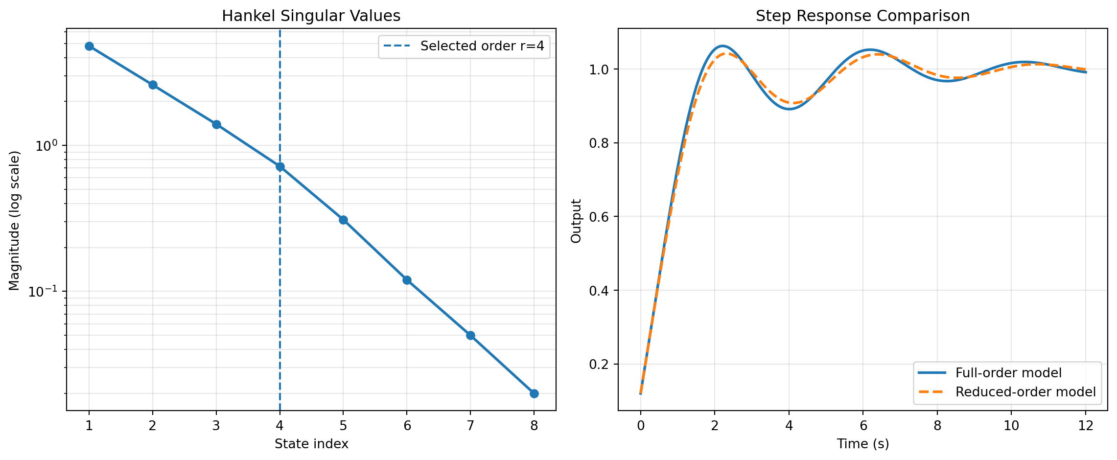
Step 2 is to inspect energetic significance. The engineer evaluates Hankel singular value behavior (directly or indirectly through reduction diagnostics) and finds a steep drop after the 4th state. This indicates that states 5–9 contribute relatively little to the measured input-output channel of interest.

Step 3 is approximation via BALRED. The team reduces from order 9 to order 4, then compares full and reduced models on:

• open-loop Bode magnitude and phase in the controller crossover range,
• step response rise/overshoot/settling,
• disturbance rejection for representative load torque changes,
• closed-loop stability margins under expected gain variation.

Step 4 is acceptance criteria. The team defines practical thresholds before deciding to adopt the reduced model: for example, phase deviation below a few degrees near crossover, settling-time error within an agreed tolerance, and no change in stability classification under planned gain schedules. If criteria fail, they raise order (for example from 4 to 5 or 6) and retest.

Step 5 is deployment alignment. The reduced model is then used for fast tuning studies and preliminary robustness sweeps. The full-order model remains the reference for final sign-off, corner-case verification, and traceability documentation.

This workflow illustrates why the two functions are complementary:

• MINREAL removes structural waste without intentionally discarding meaningful dynamics.
• BALRED performs controlled approximation to meet speed/complexity objectives.

In Boardflare terms, this maps well to a spreadsheet-first process. Analysts can start from matrix data already present in workbooks, execute reduction steps with transparent parameters (tolerance, order), and keep a documented chain from raw model to reduced model for review and governance.

How to Choose Choosing between MINREAL and BALRED is mainly about intent: exact simplification versus approximate compression.

graph TD
    A[Start with LTI model] --> B{Do you suspect redundancy?\n(pole-zero cancellation, unreachable or unobservable states)}
    B -- Yes --> C[Run MINREAL]
    B -- No --> D{Is runtime or model complexity still too high?}
    C --> D
    D -- No --> E[Keep cleaned model]
    D -- Yes --> F[Run BALRED with candidate orders]
    F --> G{Does reduced model meet response and stability checks?}
    G -- Yes --> H[Adopt reduced model for iteration/deployment]
    G -- No --> I[Increase order or revisit model scope]

Function	Primary purpose	Input style in this category	Key decision parameter	Strengths	Risks / watch-outs
MINREAL	Exact simplification to minimal realization	Transfer-function numerator/denominator data (sysdata)	tolerance	Removes non-contributing dynamics; preserves behavior when cancellation is valid; good first cleanup step	Over-aggressive tolerance can remove meaningful near-canceling dynamics; under-aggressive tolerance leaves clutter
BALRED	Approximate order reduction via balancing/truncation	State-space matrices (A, B, C, D) plus target order	order (and method choices in upstream library)	Major complexity reduction; practical for fast simulation, tuning, and embedded constraints; grounded in Hankel-energy interpretation	Reduced model is approximate; poor order choice can distort transients or frequency behavior; unstable mode handling requires careful validation

A practical decision sequence:

1. Start with MINREAL if the model source might include algebraic redundancy or noisy identification artifacts.
2. Re-evaluate model size and simulation cost after cleanup.
3. If still too large, apply BALRED and test several orders (for example r=\{2,4,6\} rather than a single guess).
4. Select the smallest order that satisfies application-specific validation criteria.

Order selection guidance for BALRED:

• Look for an elbow in Hankel singular values; cut after dominant modes.
• Prioritize fidelity around control-relevant bandwidth, not just overall fit.
• Check both open-loop and closed-loop behavior; a model that looks fine open-loop can still shift margin in feedback.
• Maintain a reproducible record of order choice rationale and validation plots.

Tolerance guidance for MINREAL:

• Begin with conservative tolerance, then increase only if obvious numerical artifacts remain.
• Compare poles/zeros before and after simplification.
• If physical interpretation of certain modes matters (e.g., resonance diagnostics), protect those modes by tightening tolerance.

In summary, MINREAL and BALRED are not substitutes; they are staged tools in a robust reduction pipeline. The first ensures the model is mathematically lean, and the second makes it computationally practical. When teams pair them with explicit acceptance tests, they gain both speed and confidence across design, analysis, and deployment workflows.

BALRED

Balanced truncation reduces a state-space model by preserving the states with the largest Hankel singular values, which represent how strongly each state contributes to input-output dynamics.

For a continuous-time linear system

\dot{x} = Ax + Bu, \quad y = Cx + Du

balanced reduction computes a transformed realization where controllability and observability Gramians are equal and diagonal, then truncates low-energy states to produce a reduced model of selected order.

This wrapper accepts stable continuous-time state-space matrices and returns the reduced realization as deterministic matrix data so the result can be compared reliably in Excel and automated tests.

Excel Usage

=BALRED(A, B, C, D, order)

• A (list[list], required): The state dynamics matrix A (NxN).
• B (list[list], required): The input matrix B (NxM).
• C (list[list], required): The output matrix C (Ny x N).
• D (list[list], required): The feedthrough matrix D (Ny x M).
• order (int, required): Desired order of the reduced model.

Returns (str): Stringified dictionary containing the reduced state-space matrices A, B, C, and D.

Example 1: Reduce stable diagonal system to order two

Inputs:

A				B	C				D	order
-1	0	0	0	1	1	1	1	1	0	2
0	-2	0	0	1
0	0	-3	0	1
0	0	0	-4	1

Excel formula:

=BALRED({-1,0,0,0;0,-2,0,0;0,0,-3,0;0,0,0,-4}, {1;1;1;1}, {1,1,1,1}, {0}, 2)

Expected output:

"{'A': [[-1.8881943210548617, -1.0094735271597388], [-1.0094735271597395, -2.396610708833071]], 'B': [[1.9213621306674076], [0.5463180989081131]], 'C': [[1.9213621306674076, 0.5463180989081124]], 'D': [[0.0]]}"

Example 2: Reduce coupled second-order system to order one

Inputs:

A		B	C		D	order
-2	1	1	1	0	0	1
-1	-3	0.5

Excel formula:

=BALRED({-2,1;-1,-3}, {1;0.5}, {1,0}, {0}, 1)

Expected output:

"{'A': [[-2.03576165455737]], 'B': [[1.0281468837336207]], 'C': [[1.0281468837336207]], 'D': [[0.0]]}"

Example 3: Reduce stable MIMO system to order two

Inputs:

A			B		C			D		order
-3	1	0	1	0	1	0	0	0	0	2
0	-2	1	0	1	0	1	1	0	0
0	0	-1	1	1

Excel formula:

=BALRED({-3,1,0;0,-2,1;0,0,-1}, {1,0;0,1;1,1}, {1,0,0;0,1,1}, {0,0;0,0}, 2)

Expected output:

"{'A': [[-0.8992182054067066, 0.30850424263019266], [-0.1383294994280792, -3.6954672181661814]], 'B': [[0.8890469932778241, 1.2443170611921701], [0.8160586847390662, -0.4681882168801548]], 'C': [[0.34033169244847766, 0.8278820677431518], [1.4909405904144586, -0.4469488396593018]], 'D': [[0.0, 0.0], [0.0, 0.0]]}"

Example 4: Request full order from already stable system

Inputs:

A		B	C		D	order
-1	0	1	1	1	0	2
0	-4	2

Excel formula:

=BALRED({-1,0;0,-4}, {1;2}, {1,1}, {0}, 2)

Expected output:

"{'A': [[-1.8936609374091684, -1.3719886811400714], [-1.3719886811400714, -3.106339062590834]], 'B': [[1.6097857971368428], [0.6392102059076513]], 'C': [[1.6097857971368423, 0.6392102059076515]], 'D': [[0.0]]}"

Python Code

Show Code

import control as ct
import numpy as np
from scipy.linalg import cholesky, solve_continuous_lyapunov, svd

def balred(A, B, C, D, order):
    """
    Balanced reduced order model of a system.

    See: https://python-control.readthedocs.io/en/latest/generated/control.balred.html

    This example function is provided as-is without any representation of accuracy.

    Args:
        A (list[list]): The state dynamics matrix A (NxN).
        B (list[list]): The input matrix B (NxM).
        C (list[list]): The output matrix C (Ny x N).
        D (list[list]): The feedthrough matrix D (Ny x M).
        order (int): Desired order of the reduced model.

    Returns:
        str: Stringified dictionary containing the reduced state-space matrices A, B, C, and D.
    """
    try:
      def to_2d_array(values, name):
        if not isinstance(values, list):
          values = [[values]]
        elif values and not isinstance(values[0], list):
          values = [[item] for item in values]

        try:
          array = np.asarray(values, dtype=float)
        except (TypeError, ValueError):
          return None, f"Error: {name} must contain only numeric values"

        if array.ndim != 2:
          return None, f"Error: {name} must be a 2D matrix"

        return array, None

      def clean_matrix(values):
        matrix = np.real_if_close(values, tol=1000)
        matrix = np.where(np.abs(matrix) < 1e-12, 0.0, matrix)
        return np.asarray(matrix, dtype=float).tolist()

      def canonicalize_state_signs(a_matrix, b_matrix, c_matrix):
        a_matrix = np.asarray(a_matrix, dtype=float).copy()
        b_matrix = np.asarray(b_matrix, dtype=float).copy()
        c_matrix = np.asarray(c_matrix, dtype=float).copy()

        for index in range(a_matrix.shape[0]):
          signature = np.concatenate((c_matrix[:, index], b_matrix[index, :], a_matrix[:, index], a_matrix[index, :]))
          significant = signature[np.abs(signature) > 1e-12]
          if significant.size and significant[0] < 0:
            a_matrix[:, index] *= -1
            a_matrix[index, :] *= -1
            b_matrix[index, :] *= -1
            c_matrix[:, index] *= -1

        return a_matrix, b_matrix, c_matrix

      A_mat, error = to_2d_array(A, "A")
      if error:
        return error
      B_mat, error = to_2d_array(B, "B")
      if error:
        return error
      C_mat, error = to_2d_array(C, "C")
      if error:
        return error
      D_mat, error = to_2d_array(D, "D")
      if error:
        return error

      nstates = A_mat.shape[0]
      if nstates == 0 or A_mat.shape[1] != nstates:
        return "Error: A must be a non-empty square matrix"

      if B_mat.shape[0] != nstates:
        return "Error: B must have the same number of rows as A"

      if C_mat.shape[1] != nstates:
        return "Error: C must have the same number of columns as A"

      if D_mat.shape != (C_mat.shape[0], B_mat.shape[1]):
        return "Error: D must have dimensions compatible with B and C"

      desired_order = int(order)
      if desired_order < 1 or desired_order > nstates:
        return "Error: order must be between 1 and the number of states in A"

      eigenvalues = np.linalg.eigvals(A_mat)
      if np.any(np.real(eigenvalues) >= 0):
        return "Error: balanced reduction requires a stable continuous-time A matrix"

      try:
        system = ct.ss(A_mat.tolist(), B_mat.tolist(), C_mat.tolist(), D_mat.tolist())
        reduced = ct.balred(system, desired_order)
        a_red = np.asarray(reduced.A, dtype=float)
        b_red = np.asarray(reduced.B, dtype=float)
        c_red = np.asarray(reduced.C, dtype=float)
        d_red = np.asarray(reduced.D, dtype=float)
      except Exception:
        gram_controllability = solve_continuous_lyapunov(A_mat, -(B_mat @ B_mat.T))
        gram_observability = solve_continuous_lyapunov(A_mat.T, -(C_mat.T @ C_mat))
        gram_controllability = 0.5 * (gram_controllability + gram_controllability.T)
        gram_observability = 0.5 * (gram_observability + gram_observability.T)

        factor_controllability = cholesky(gram_controllability, lower=True)
        factor_observability = cholesky(gram_observability, lower=True)
        left_vectors, singular_values, right_vectors_h = svd(
          factor_observability.T @ factor_controllability
        )

        if np.any(singular_values[:desired_order] <= 0):
          return "Error: system must be controllable and observable for balanced reduction"

        sigma_inv_sqrt = np.diag(1.0 / np.sqrt(singular_values))
        transform = factor_controllability @ right_vectors_h.T @ sigma_inv_sqrt
        inverse_transform = sigma_inv_sqrt @ left_vectors.T @ factor_observability.T

        balanced_a = inverse_transform @ A_mat @ transform
        balanced_b = inverse_transform @ B_mat
        balanced_c = C_mat @ transform

        a_red = balanced_a[:desired_order, :desired_order]
        b_red = balanced_b[:desired_order, :]
        c_red = balanced_c[:, :desired_order]
        d_red = D_mat

      a_red, b_red, c_red = canonicalize_state_signs(a_red, b_red, c_red)

      return str({
        "A": clean_matrix(a_red),
        "B": clean_matrix(b_red),
        "C": clean_matrix(c_red),
        "D": clean_matrix(d_red),
      })
    except Exception as e:
        return f"Error: {str(e)}"

Online Calculator

A *

The state dynamics matrix A (NxN).

B *

The input matrix B (NxM).

C *

The output matrix C (Ny x N).

D *

The feedthrough matrix D (Ny x M).

order *

Desired order of the reduced model.

---

MINREAL

Minimal realization removes redundant dynamics while preserving the input-output behavior of a linear system.

For transfer-function models, this operation cancels pole-zero pairs that are numerically close within a tolerance, yielding an equivalent lower-order representation. For state-space models, it removes uncontrollable and unobservable states.

In transfer-function form,

G(s) = \frac{N(s)}{D(s)}

common factors of N(s) and D(s) are canceled to obtain a simplified model with the same external response.

Excel Usage

=MINREAL(sysdata, tolerance)

• sysdata (list[list], required): Numerator and denominator of the system to simplify.
• tolerance (float, optional, default: null): Tolerance for state elimination or pole-zero cancellation.

Returns (str): Stringified dictionary containing the numerator and denominator coefficients of the minimal transfer function.

Example 1: Pole-zero cancellation

Inputs:

sysdata		tolerance
1	1
1	2

Excel formula:

=MINREAL({1,1;1,2,1}, )

Expected output:

"{'num': [1.0], 'den': [1.0, 1.0]}"

Example 2: Exact cancellation to first-order model

Inputs:

sysdata			tolerance
1	3	2
1	4	5

Excel formula:

=MINREAL({1,3,2;1,4,5,2}, )

Expected output:

"{'num': [1.0], 'den': [1.0, 0.9999999999999997]}"

Example 3: No cancellation keeps second-order dynamics

Inputs:

sysdata	tolerance
1
1

Excel formula:

=MINREAL({1;1,2,2}, )

Expected output:

"{'num': [1.0], 'den': [1.0, 1.9999999999999996, 1.9999999999999991]}"

Example 4: Near cancellation with explicit tolerance

Inputs:

sysdata			tolerance
1	2.0001	1.0001	0.001
1	2	1

Excel formula:

=MINREAL({1,2.0001,1.0001;1,2,1}, 0.001)

Expected output:

"{'num': [1.0], 'den': [1.0]}"

Python Code

Show Code

import control as ct
import numpy as np

def minreal(sysdata, tolerance=None):
    """
    Eliminate uncontrollable or unobservable states.

    See: https://python-control.readthedocs.io/en/latest/generated/control.minreal.html

    This example function is provided as-is without any representation of accuracy.

    Args:
        sysdata (list[list]): Numerator and denominator of the system to simplify.
        tolerance (float, optional): Tolerance for state elimination or pole-zero cancellation. Default is None.

    Returns:
        str: Stringified dictionary containing the numerator and denominator coefficients of the minimal transfer function.
    """
    try:
        def clean_coefficients(values):
            coefficients = np.atleast_1d(np.asarray(values, dtype=float)).flatten()
            coefficients = np.real_if_close(coefficients, tol=1000)
            coefficients = np.where(np.abs(coefficients) < 1e-12, 0.0, coefficients)
            return np.asarray(coefficients, dtype=float).tolist()

        def to_tf(data):
            if not isinstance(data, list) or len(data) != 2:
                return None
            try:
                num_row = data[0] if isinstance(data[0], list) else [data[0]]
                den_row = data[1] if isinstance(data[1], list) else [data[1]]
                num = [float(v) for v in num_row]
                den = [float(v) for v in den_row]
            except (TypeError, ValueError):
                return None
            if not num or not den:
                return None
            return ct.tf(num, den)

        sys = to_tf(sysdata)
        if sys is None:
            return "Error: sysdata must contain numeric numerator and denominator rows"

        tol = float(tolerance) if tolerance is not None else None
        if tol is not None and tol < 0:
            return "Error: tolerance must be non-negative"

        res = ct.minreal(sys, tol=tol, verbose=False)
        numerator = clean_coefficients(res.num[0][0])
        denominator = clean_coefficients(res.den[0][0])
        return str({"num": numerator, "den": denominator})
    except Exception as e:
        return f"Error: {str(e)}"

Online Calculator

sysdata *

Numerator and denominator of the system to simplify.

tolerance

Tolerance for state elimination or pole-zero cancellation.