Wavelets
Overview
Introduction
Wavelet analysis is a multi-resolution signal analysis framework that represents a signal using short, localized basis functions instead of infinitely long sinusoids. In practical terms, wavelets answer a question that standard spectral methods often cannot answer cleanly: what frequency-like behavior occurs, and when does it occur? This makes wavelets central to modern condition monitoring, vibration diagnostics, seismic interpretation, biomedical signal processing, image compression, denoising, and transient-event detection. For formal background, see Wavelet.
In engineering and analytics workflows, signals are rarely stationary. Motor current has startup transients, pressure traces include valve events, seismic traces include reflections at specific times, and biomedical traces contain bursts and artifacts. A pure Fourier workflow can identify global spectral content but loses temporal localization. Wavelets maintain both scale (frequency-like) and time localization, which is why they are a practical workhorse for event-rich data.
This category combines two mature Python ecosystems:
- SciPy signal processing, used here for core wavelet and filter utilities such as CWT, RICKER, MORLET2, DAUB, QMF, and CASCADE.
- PyWavelets, used for production discrete wavelet decomposition and coefficient post-processing through WAVEDEC and THRESHOLD.
Together, these tools support two complementary analysis styles:
- Continuous, exploratory time-scale analysis for feature discovery and transient localization using CWT and prototype wavelets (RICKER, MORLET2).
- Discrete, model-building and denoising workflows using WAVEDEC, coefficient filtering with THRESHOLD, and wavelet/filter construction support via DAUB, QMF, and CASCADE.
From a business perspective, wavelets matter because they reduce false alarms and missed events in operational monitoring. Instead of reacting to noisy threshold crossings in raw time series, teams can analyze structured coefficient patterns across scales, isolate anomalies, and prioritize interventions. In finance and market microstructure, they support multi-horizon decomposition; in energy and manufacturing, they separate baseline drift from fault signatures; in geoscience, they highlight localized reflection behavior. The practical advantage is the same: higher signal-to-noise insight without requiring users to abandon spreadsheet-centric workflows.
When to Use It
Wavelet tools are most valuable when the job is not simply “compute a frequency spectrum,” but rather “understand changing behavior across time and scale.” They are especially useful when the signal contains abrupt changes, intermittent bursts, nonstationary structure, or mixed low/high-frequency phenomena.
Use wavelets for the following jobs-to-be-done:
- Detect and localize transient events in operational signals
- Scenario: A reliability engineer monitors pump vibration and wants to pinpoint cavitation bursts, bearing defects, or startup anomalies that occur briefly.
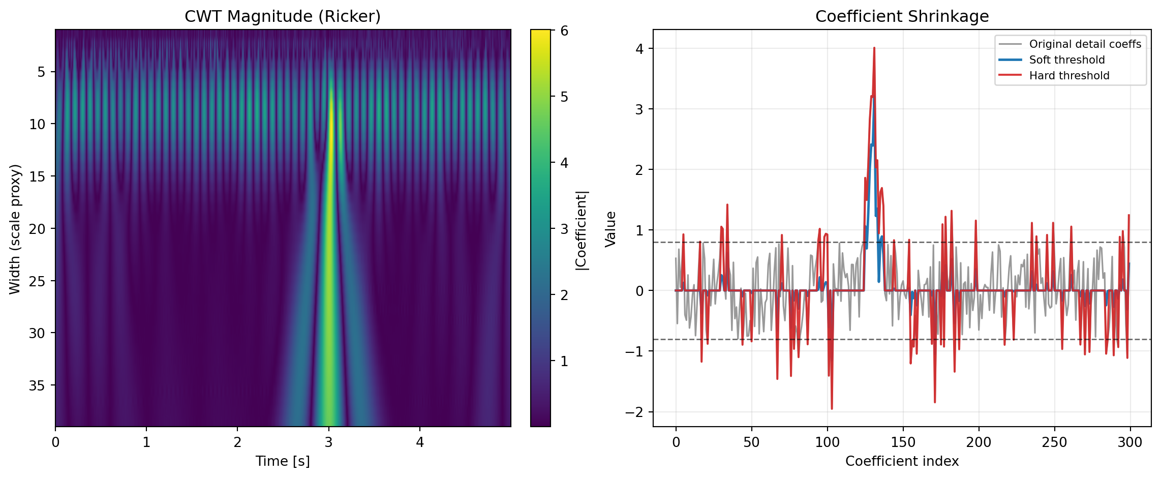
- Why wavelets: CWT generates a scale-by-time coefficient map where short events become localized ridges; RICKER often works well for impulse-like events, while MORLET2 is better when oscillatory structure is important.
- Outcome: Faster root-cause triage because event timing and characteristic scale are visible simultaneously.
- Denoise measured signals while preserving edges and meaningful discontinuities
- Scenario: A process engineer receives noisy sensor data (flow, pressure, acoustic emission) and needs a cleaner signal for downstream control logic.
- Why wavelets: WAVEDEC separates coarse trends from scale-specific details. Small detail coefficients are likely noise and can be attenuated with THRESHOLD in soft, hard, garrote, greater, or less modes.
- Outcome: Better denoising than simple moving averages because sharp events and edges are preserved more effectively.
- Design and validate discrete wavelet filter banks for custom analysis pipelines
- Scenario: A signal-processing developer needs reproducible low-pass/high-pass analysis filters for a custom DWT implementation or educational verification.
- Why wavelets: DAUB returns Daubechies low-pass coefficients, QMF derives quadrature mirror high-pass coefficients, and CASCADE visualizes resulting scaling/wavelet functions on dyadic grids.
- Outcome: Transparent filter-bank construction with less implementation error and clearer auditability.
- Separate long-horizon trend from short-horizon variation for multiscale decisions
- Scenario: Teams analyzing demand, energy load, traffic, or machine telemetry need to distinguish baseline changes from short-lived fluctuations.
- Why wavelets: WAVEDEC naturally provides approximation and detail coefficients across levels; each level corresponds to a different effective scale band.
- Outcome: More robust forecasting features and intervention logic by using scale-aware components rather than raw series alone.
Wavelets are usually preferred over purely global spectral methods when assumptions of stationarity are weak. They are also preferred over basic smoothing when preserving local structure is important. If the data is highly stationary and only global spectral peaks matter, classical Fourier methods may be simpler. If the objective is local events, multiscale denoising, or boundary-aware decomposition, this category is usually the better fit.
How It Works
Wavelet analysis relies on translations and dilations of a mother wavelet \psi(t) and (for discrete orthogonal transforms) a scaling function \phi(t). The continuous wavelet transform of a signal x(t) is
W_x(a,b) = \frac{1}{\sqrt{|a|}}\int_{-\infty}^{\infty} x(t)\,\psi^*\!\left(\frac{t-b}{a}\right) dt,
where a is scale and b is translation. Small a captures short-duration/high-frequency behavior; large a captures long-duration/low-frequency behavior.
For practical sampled data, CWT computes this over a finite set of widths/scales and returns a coefficient matrix. In this category, users choose wavelet family behavior through wavelet_type (notably Ricker or Morlet2), then inspect coefficient magnitude patterns over scale and time.
The discrete wavelet transform (DWT), used by WAVEDEC, is filter-bank based. At each level j, approximation and detail coefficients are generated by convolution and downsampling:
cA_j[k] = \sum_n x_j[n] h[2k-n], \qquad cD_j[k] = \sum_n x_j[n] g[2k-n],
with analysis low-pass filter h and high-pass filter g, and x_{j+1}=cA_j. Repeating this yields multilevel decomposition:
[cA_n, cD_n, cD_{n-1}, \ldots, cD_1].
This representation is efficient and interpretable: coarse approximation coefficients summarize low-frequency structure, while detail coefficients capture progressively finer dynamics.
Conceptual role of each function in the category
Although the page is organized by calculators, the tools map to clear conceptual roles:
- Prototype and filter construction
- Wavelet generation for CWT and interpretability
- Transform and coefficient processing
Thresholding theory in denoising workflows
After decomposition, many noise models assume high-frequency small-magnitude coefficients are mostly noise. Thresholding applies an operator T_\lambda(\cdot) with threshold \lambda:
- Soft threshold:
T_\lambda^{\text{soft}}(x)=\operatorname{sign}(x)\max(|x|-\lambda,0)
- Hard threshold:
T_\lambda^{\text{hard}}(x)= \begin{cases} x, & |x|\ge \lambda\\ 0, & |x|<\lambda \end{cases}
In practice, THRESHOLD provides multiple modes (soft/hard/garrote/greater/less), which is useful when users need either smooth shrinkage, strict cutoff behavior, or directional filtering behavior.
Boundary conditions and practical assumptions
Any finite signal transform must define edge behavior. WAVEDEC exposes wavedec_mode (e.g., symmetric, periodization, zero). This choice matters:
symmetricoften performs well for many physical signals by reducing edge discontinuity artifacts.periodizationis useful when periodic assumptions are justified.zerocan bias boundaries for nonzero edge levels.
Additional practical assumptions:
- Sampling should be dense enough to capture target dynamics.
- Width/level choices should align with known event durations or frequency bands.
- Coefficient interpretation should account for scale-dependent amplitude behavior.
- Threshold values should be validated against signal-to-noise goals, not chosen arbitrarily.
The implementation stack is robust and transparent: SciPy Signal provides foundational routines for wavelet shapes and CWT utilities; PyWavelets DWT docs and PyWavelets thresholding docs provide decomposition and denoising primitives designed for production use.
Practical Example
Consider a rotating-equipment monitoring workflow where a plant engineer receives a 1 kHz vibration signal from a pump and needs to identify intermittent bearing impacts while generating a cleaner trend for control and reporting.
Step 1: Explore event localization with CWT
- Load the signal into the CWT calculator.
- Start with
wavelet_type="ricker"and a width range that spans expected event durations. - Inspect coefficient rows for concentrated bursts at specific times and scales.
If impacts are strongly oscillatory rather than spike-like, switch to wavelet_type="morlet2" in CWT. When needed, generate a custom reference wavelet shape with MORLET2 to confirm parameterization (s_width, w_omega) and interpret effective time-frequency concentration.
Step 2: Build a multilevel decomposition for denoising and features
- Send the same signal to WAVEDEC with a wavelet such as
db4orsym5. - Use
wavedec_mode="symmetric"initially. - Choose
levelbased on sample length and target feature scales (or leave empty for max valid level).
This returns [cA_n, cD_n, ..., cD1] as rows. Coarse approximation (cA_n) captures baseline motion/trend; detail levels isolate progressively finer behavior.
Step 3: Suppress noise in detail coefficients
- Apply THRESHOLD to selected detail coefficient ranges.
- Start with
threshold_mode="soft"for smoother denoising. - Increase/decrease
valueuntil residual noise is reduced without erasing fault-relevant bursts.
For stricter retention of high-amplitude impacts, test threshold_mode="hard". If process constraints require directional replacement logic, greater and less modes can be used in post-processing pipelines.
Step 4: Validate the wavelet/filter basis if needed
When teams require deeper verification of filter behavior (for algorithm QA, education, or custom implementation):
- Use DAUB to generate low-pass coefficients for a target order.
- Use QMF to derive the corresponding high-pass coefficients.
- Use CASCADE to inspect \phi and \psi over dyadic points and confirm expected smoothness/support behavior.
This is especially useful when teams need explainability documentation for regulated workflows or model governance.
Step 5: Operationalize decision rules
- Track coefficient energy over selected scales as a health indicator.
- Use reconstructed or denoised signals for alarm logic to reduce nuisance trips.
- Compare baseline periods vs fault periods at matched decomposition levels.
Compared with traditional Excel-only moving-average and FFT-only workflows, this wavelet pipeline gives better temporal localization, better edge-preserving denoising, and clearer multiscale diagnostics. It supports both rapid exploratory analysis and disciplined, repeatable production decisions.
How to Choose
Choosing the right calculator is mainly about objective: explore time-scale structure, decompose for denoising/features, or construct/inspect wavelet filters. The table below provides a direct selection map.
| Function | Best for | Inputs to decide carefully | Strengths | Trade-offs |
|---|---|---|---|---|
| CWT | Time-localized multiscale exploration | widths, wavelet_type |
Excellent transient localization; intuitive scale-time map | More computationally intensive; coefficient interpretation depends on width choice |
| RICKER | Real wavelet kernel for impulse-like events | points, a_width |
Simple and robust for spikes/edges | Less phase-rich than complex wavelets |
| MORLET2 | Complex oscillatory wavelet kernel | m_points, s_width, w_omega |
Better for oscillatory bursts and phase-sensitive analysis | Parameter tuning required; output is complex-valued representation |
| WAVEDEC | Multilevel DWT decomposition | wavelet, wavedec_mode, level |
Fast, compact coefficients; excellent for denoising/features | Requires thoughtful mode/level choice near boundaries |
| THRESHOLD | Coefficient denoising and selection | value, threshold_mode, substitute |
Flexible shrinkage rules; easy workflow integration | Over-thresholding can remove useful detail |
| DAUB | Retrieve Daubechies low-pass taps | p |
Standard orthogonal wavelet filter coefficients | Focused utility; not a full transform by itself |
| QMF | Derive high-pass mirror filter | hk |
Quick construction of analysis/synthesis pair component | Assumes valid low-pass prototype input |
| CASCADE | Inspect scaling/wavelet functions from filters | hk, J |
Strong for validation, education, and filter QA | Diagnostic/constructive tool, not end-user transform output |
Use this decision flow when starting from a business problem:
graph TD
     A[Start: What is the analysis goal?] --> B{Need time-localized event map?}
     B -- Yes --> C[Use CWT]
     C --> D{Event shape?}
     D -- Impulse-like --> E[Use RICKER or CWT wavelet_type=ricker]
     D -- Oscillatory --> F[Use MORLET2 or CWT wavelet_type=morlet2]

     B -- No --> G{Need denoising or multiscale features?}
     G -- Yes --> H[Use WAVEDEC]
     H --> I[Apply THRESHOLD to detail coefficients]

     G -- No --> J{Need filter-bank construction/validation?}
     J -- Yes --> K[Use DAUB for low-pass taps]
     K --> L[Use QMF for high-pass taps]
     L --> M[Use CASCADE to inspect phi/psi]
     J -- No --> N[Re-check problem framing or use broader signal-processing tools]
Practical selection guidance:
- Choose CWT first when diagnosing unknown transient behavior.
- Choose WAVEDEC first when building repeatable denoising or predictive features.
- Choose THRESHOLD mode based on tolerance for coefficient bias:
softfor smoother shrinkage,hardfor strict retention,garrotefor intermediate behavior. - Choose DAUB, QMF, and CASCADE when implementation transparency and filter construction checks are part of the deliverable.
In short, this category is strongest when teams need a bridge between exploratory signal insight and production-grade multiscale processing. By pairing SciPy-based wavelet primitives with PyWavelets decomposition and thresholding, the workflow supports both fast diagnosis and robust operational deployment.
CASCADE
The cascade algorithm (also known as the vector cascade algorithm) iteratively computes the values of the scaling function (phi) and the wavelet function (psi) at dyadic points starting from the filter coefficients.
The resulting functions are vital for constructing discrete wavelet transforms.
Excel Usage
=CASCADE(hk, J)hk(list[list], required): Coefficients of the low-pass filter (Excel range).J(int, optional, default: 7): Number of iterations (level of resolution). Higher J means denser grid.
Returns (list[list]): A 2D array where the first row is the dyadic grid points, the second is phi(x), and the third is psi(x).
Example 1: Daubechies order 2 cascade
Inputs:
| hk | J | |||
|---|---|---|---|---|
| 0.48296291 | 0.8365163 | 0.22414387 | -0.12940952 | 2 |
Excel formula:
=CASCADE({0.48296291,0.8365163,0.22414387,-0.12940952}, 2)Expected output:
| Result | |||||||||||
|---|---|---|---|---|---|---|---|---|---|---|---|
| 0 | 0.25 | 0.5 | 0.75 | 1 | 1.25 | 1.5 | 1.75 | 2 | 2.25 | 2.5 | 2.75 |
| 0 | 0.63726 | 0.933013 | 1.10377 | 1.36603 | 0.341506 | 1.14347e-8 | -0.0915063 | -0.366025 | 0.0212341 | 0.0669873 | -0.0122595 |
| 0 | -0.170753 | -0.25 | -0.295753 | -0.366025 | 1.09151 | 1.73205 | -0.658494 | -1.36603 | 0.0792468 | 0.25 | -0.0457532 |
Python Code
Show Code
import numpy as np
from scipy.signal import cascade as scipy_cascade

def cascade(hk, J=7):
    """
    Compute scaling and wavelet functions at dyadic points from filter coefficients.

    See: https://docs.scipy.org/doc/scipy/reference/generated/scipy.signal.cascade.html

    This example function is provided as-is without any representation of accuracy.

    Args:
        hk (list[list]): Coefficients of the low-pass filter (Excel range).
        J (int, optional): Number of iterations (level of resolution). Higher J means denser grid. Default is 7.

    Returns:
        list[list]: A 2D array where the first row is the dyadic grid points, the second is phi(x), and the third is psi(x).
    """
    try:
        def to_1d(v):
            if isinstance(v, list):
                return np.array([float(x) for row in v for x in row])
            return np.array([float(v)])

        hk_arr = to_1d(hk)

        x, phi, psi = scipy_cascade(hk_arr, J=int(J))

        return [x.tolist(), phi.tolist(), psi.tolist()]
    except Exception as e:
        return f"Error: {str(e)}"
Online Calculator
Coefficients of the low-pass filter (Excel range).
Number of iterations (level of resolution). Higher J means denser grid.
CWT
The Continuous Wavelet Transform (CWT) is a time-frequency analysis tool that decomposes a signal into wavelets. Unlike the Fourier transform, wavelets are localized in both time and frequency.
This implementation uses the specified wavelet function and widths to produce a 2D matrix of coefficients.
Excel Usage
=CWT(data, widths, wavelet_type)data(list[list], required): The input signal data.widths(list[list], required): Sequence of widths to use for the transform.wavelet_type(str, optional, default: “ricker”): The wavelet function to use.
Returns (list[list]): A 2D matrix of transform coefficients (widths as rows, data as columns).
Example 1: Ricker CWT
Inputs:
| data | widths | wavelet_type | ||||||||
|---|---|---|---|---|---|---|---|---|---|---|
| 1 | 2 | 3 | 4 | 3 | 2 | 1 | 1 | 2 | 3 | ricker |
Excel formula:
=CWT({1,2,3,4,3,2,1}, {1,2,3}, "ricker")Expected output:
| Result | ||||||
|---|---|---|---|---|---|---|
| -0.497416 | 0.0948513 | 1.03926 | 1.90658 | 1.03926 | 0.0948513 | -0.497416 |
| 0.4296 | 2.10362 | 3.77763 | 4.39092 | 3.77763 | 2.10362 | 0.4296 |
| 2.01115 | 3.57677 | 4.91964 | 5.42039 | 4.91964 | 3.57677 | 2.01115 |
Python Code
Show Code
import numpy as np
from scipy.signal import cwt as scipy_cwt
from scipy.signal import ricker, morlet2

def cwt(data, widths, wavelet_type='ricker'):
    """
    Perform a Continuous Wavelet Transform (CWT).

    See: https://docs.scipy.org/doc/scipy/reference/generated/scipy.signal.cwt.html

    This example function is provided as-is without any representation of accuracy.

    Args:
        data (list[list]): The input signal data.
        widths (list[list]): Sequence of widths to use for the transform.
        wavelet_type (str, optional): The wavelet function to use. Valid options: Ricker, Morlet 2. Default is 'ricker'.

    Returns:
        list[list]: A 2D matrix of transform coefficients (widths as rows, data as columns).
    """
    try:
        def to_1d(v):
            if isinstance(v, list):
                return np.array([float(x) for row in v for x in row])
            return np.array([float(v)])

        data_arr = to_1d(data)
        widths_arr = to_1d(widths)

        # Map wavelet_type string to function
        wavelet_map = {
            'ricker': ricker,
            'morlet2': morlet2
        }
        wav_func = wavelet_map.get(wavelet_type, ricker)

        # Determine if output should be complex
        out_dtype = np.float64
        if wavelet_type == 'morlet2':
            out_dtype = np.complex128

        result = scipy_cwt(data_arr, wav_func, widths_arr, dtype=out_dtype)

        if wavelet_type == 'morlet2':
            return np.abs(result).tolist()

        return result.tolist()
    except Exception as e:
        return f"Error: {str(e)}"
Online Calculator
The input signal data.
Sequence of widths to use for the transform.
The wavelet function to use.
DAUB
Daubechies wavelets are a family of orthogonal wavelets defining a discrete wavelet transform. They are characterized by a maximum number of vanishing moments for some given support.
This function returns the coefficients of the low-pass filter for the wavelet of order p.
Excel Usage
=DAUB(p)p(int, required): Order of the zero at f=1/2 (from 1 to 34).
Returns (list[list]): A 1D array (as a row) of filter coefficients.
Example 1: Daub order 2
Inputs:
| p |
|---|
| 2 |
Excel formula:
=DAUB(2)Expected output:
| Result | |||
|---|---|---|---|
| 0.482963 | 0.836516 | 0.224144 | -0.12941 |
Example 2: Daub order 4
Inputs:
| p |
|---|
| 4 |
Excel formula:
=DAUB(4)Expected output:
| Result | |||||||
|---|---|---|---|---|---|---|---|
| 0.230378 | 0.714847 | 0.630881 | -0.0279838 | -0.187035 | 0.0308414 | 0.032883 | -0.0105974 |
Python Code
Show Code
import numpy as np
from scipy.signal import daub as scipy_daub

def daub(p):
    """
    Get coefficients for the low-pass filter producing Daubechies wavelets.

    See: https://docs.scipy.org/doc/scipy/reference/generated/scipy.signal.daub.html

    This example function is provided as-is without any representation of accuracy.

    Args:
        p (int): Order of the zero at f=1/2 (from 1 to 34).

    Returns:
        list[list]: A 1D array (as a row) of filter coefficients.
    """
    try:
        result = scipy_daub(int(p))
        return [result.tolist()]
    except Exception as e:
        return f"Error: {str(e)}"
Online Calculator
Order of the zero at f=1/2 (from 1 to 34).
MORLET2
The Morlet wavelet is a complex sinusoid modulated by a Gaussian envelope. It provides an excellent balance between time and frequency localization and is widely used in continuous wavelet transforms.
This version (morlet2) is designed for direct use with the CWT function.
Excel Usage
=MORLET2(m_points, s_width, w_omega)m_points(int, required): Length of the wavelet (number of points).s_width(float, required): Width parameter of the wavelet.w_omega(float, optional, default: 5): Omega0 (central frequency parameter).
Returns (list[list]): A 1D array of the complex Morlet wavelet (interleaved real and imaginary).
Example 1: Basic Morlet2
Inputs:
| m_points | s_width | w_omega |
|---|---|---|
| 24 | 4 | 2 |
Excel formula:
=MORLET2(24, 4, 2)Expected output:
| Result | |||||||||||||||||||||||
|---|---|---|---|---|---|---|---|---|---|---|---|---|---|---|---|---|---|---|---|---|---|---|---|
| 0.00518711 | 0.00613401 | 0.00084149 | -0.0175205 | -0.0531354 | -0.099706 | -0.134882 | -0.125295 | -0.0456509 | 0.0974124 | 0.256137 | 0.361056 | 0.361056 | 0.256137 | 0.0974124 | -0.0456509 | -0.125295 | -0.134882 | -0.099706 | -0.0531354 | -0.0175205 | 0.00084149 | 0.00613401 | 0.00518711 |
| 0.00306145 | 0.0102887 | 0.022363 | 0.0351516 | 0.0370115 | 0.0108514 | -0.055695 | -0.155194 | -0.25201 | -0.293169 | -0.238617 | -0.0921926 | 0.0921926 | 0.238617 | 0.293169 | 0.25201 | 0.155194 | 0.055695 | -0.0108514 | -0.0370115 | -0.0351516 | -0.022363 | -0.0102887 | -0.00306145 |
Python Code
Show Code
import numpy as np
from scipy.signal import morlet2 as scipy_morlet2

def morlet2(m_points, s_width, w_omega=5):
    """
    Generate a complex Morlet wavelet for a given length and width.

    See: https://docs.scipy.org/doc/scipy/reference/generated/scipy.signal.morlet2.html

    This example function is provided as-is without any representation of accuracy.

    Args:
        m_points (int): Length of the wavelet (number of points).
        s_width (float): Width parameter of the wavelet.
        w_omega (float, optional): Omega0 (central frequency parameter). Default is 5.

    Returns:
        list[list]: A 1D array of the complex Morlet wavelet (interleaved real and imaginary).
    """
    try:
        result = scipy_morlet2(int(m_points), float(s_width), w=float(w_omega))
        # Return interleaved real and imag
        return [result.real.tolist(), result.imag.tolist()]
    except Exception as e:
        return f"Error: {str(e)}"
Online Calculator
Length of the wavelet (number of points).
Width parameter of the wavelet.
Omega0 (central frequency parameter).
QMF
A Quadrature Mirror Filter (QMF) is a pair of filters that decompose a signal into two subbands (low-pass and high-pass) and allow for perfect reconstruction of the original signal.
This function generates the high-pass filter coefficients from the provided low-pass filter coefficients.
Excel Usage
=QMF(hk)hk(list[list], required): Coefficients of the low-pass filter (Excel range).
Returns (list[list]): A 1D array (as a row) of high-pass filter coefficients.
Example 1: Simple QMF
Inputs:
| hk | |
|---|---|
| 1 | 1 |
Excel formula:
=QMF({1,1})Expected output:
| Result | |
|---|---|
| 1 | -1 |
Python Code
Show Code
import numpy as np
from scipy.signal import qmf as scipy_qmf

def qmf(hk):
    """
    Return a Quadrature Mirror Filter (QMF) from low-pass coefficients.

    See: https://docs.scipy.org/doc/scipy/reference/generated/scipy.signal.qmf.html

    This example function is provided as-is without any representation of accuracy.

    Args:
        hk (list[list]): Coefficients of the low-pass filter (Excel range).

    Returns:
        list[list]: A 1D array (as a row) of high-pass filter coefficients.
    """
    try:
        def to_1d(v):
            if isinstance(v, list):
                return np.array([float(x) for row in v for x in row])
            return np.array([float(v)])

        hk_arr = to_1d(hk)
        result = scipy_qmf(hk_arr)
        return [result.tolist()]
    except Exception as e:
        return f"Error: {str(e)}"
Online Calculator
Coefficients of the low-pass filter (Excel range).
RICKER
The Ricker wavelet is a real-valued wavelet modeled as the negative second derivative of a Gaussian function.
It is commonly used in seismic and geophysical applications, as well as in edge detection in image processing.
Excel Usage
=RICKER(points, a_width)points(int, required): Number of points in the vector.a_width(float, required): Width parameter of the wavelet.
Returns (list[list]): A 1D array (as a row) of the Ricker wavelet.
Example 1: Basic Ricker
Inputs:
| points | a_width |
|---|---|
| 24 | 4 |
Excel formula:
=RICKER(24, 4)Expected output:
| Result | |||||||||||||||||||||||
|---|---|---|---|---|---|---|---|---|---|---|---|---|---|---|---|---|---|---|---|---|---|---|---|
| -0.0505321 | -0.0814766 | -0.119917 | -0.159441 | -0.1881 | -0.190001 | -0.150073 | -0.0611778 | 0.0693122 | 0.217377 | 0.347375 | 0.423565 | 0.423565 | 0.347375 | 0.217377 | 0.0693122 | -0.0611778 | -0.150073 | -0.190001 | -0.1881 | -0.159441 | -0.119917 | -0.0814766 | -0.0505321 |
Python Code
Show Code
import numpy as np
from scipy.signal import ricker as scipy_ricker

def ricker(points, a_width):
    """
    Return a Ricker wavelet (Mexican hat wavelet).

    See: https://docs.scipy.org/doc/scipy/reference/generated/scipy.signal.ricker.html

    This example function is provided as-is without any representation of accuracy.

    Args:
        points (int): Number of points in the vector.
        a_width (float): Width parameter of the wavelet.

    Returns:
        list[list]: A 1D array (as a row) of the Ricker wavelet.
    """
    try:
        result = scipy_ricker(int(points), float(a_width))
        return [result.tolist()]
    except Exception as e:
        return f"Error: {str(e)}"
Online Calculator
Number of points in the vector.
Width parameter of the wavelet.
THRESHOLD
This function applies wavelet-style thresholding to each value in an input range. Values are modified according to a selected thresholding rule and a threshold magnitude.
In soft thresholding, values are shrunk toward zero by the threshold after sign preservation, while in hard thresholding values below the threshold are replaced by a substitute value. Additional modes include garrote, greater, and less thresholding rules.
For soft thresholding, an input value x and threshold \lambda produce:
\hat{x} = \operatorname{sign}(x)\max(|x|-\lambda, 0)
This enables denoising workflows by attenuating small-magnitude coefficients.
Excel Usage
=THRESHOLD(data, value, threshold_mode, substitute)data(list[list], required): Input numeric values as an Excel range.value(float, required): Threshold value.threshold_mode(str, optional, default: “soft”): Thresholding mode.substitute(float, optional, default: 0): Replacement value for thresholded entries.
Returns (list[list]): Thresholded values in a 2D range matching the input shape.
Example 1: Soft threshold on a single row
Inputs:
| data | value | threshold_mode | substitute | ||||
|---|---|---|---|---|---|---|---|
| 1 | 1.5 | 2 | 2.5 | 3 | 2 | soft | 0 |
Excel formula:
=THRESHOLD({1,1.5,2,2.5,3}, 2, "soft", 0)Expected output:
| Result | ||||
|---|---|---|---|---|
| 0 | 0 | 0 | 0.5 | 1 |
Example 2: Hard threshold on a 2x3 matrix
Inputs:
| data | value | threshold_mode | substitute | ||
|---|---|---|---|---|---|
| 1 | 2 | 3 | 2 | hard | 0 |
| 4 | 0.5 | 2.5 |
Excel formula:
=THRESHOLD({1,2,3;4,0.5,2.5}, 2, "hard", 0)Expected output:
| Result | ||
|---|---|---|
| 0 | 2 | 3 |
| 4 | 0 | 2.5 |
Example 3: Greater mode replaces values below threshold
Inputs:
| data | value | threshold_mode | substitute | |||
|---|---|---|---|---|---|---|
| 1 | 2 | 3 | 4 | 2.5 | greater | -1 |
Excel formula:
=THRESHOLD({1,2,3,4}, 2.5, "greater", -1)Expected output:
| Result | |||
|---|---|---|---|
| -1 | -1 | 3 | 4 |
Example 4: Less mode replaces values above threshold
Inputs:
| data | value | threshold_mode | substitute | |||
|---|---|---|---|---|---|---|
| 1 | 2 | 3 | 4 | 2.5 | less | 9 |
Excel formula:
=THRESHOLD({1,2,3,4}, 2.5, "less", 9)Expected output:
| Result | |||
|---|---|---|---|
| 1 | 2 | 9 | 9 |
Python Code
Show Code
import numpy as np
import pywt

def threshold(data, value, threshold_mode='soft', substitute=0):
    """
    Apply elementwise wavelet thresholding to numeric data.

    See: https://pywavelets.readthedocs.io/en/latest/ref/thresholding-functions.html

    This example function is provided as-is without any representation of accuracy.

    Args:
        data (list[list]): Input numeric values as an Excel range.
        value (float): Threshold value.
        threshold_mode (str, optional): Thresholding mode. Valid options: Soft, Hard, Garrote, Greater, Less. Default is 'soft'.
        substitute (float, optional): Replacement value for thresholded entries. Default is 0.

    Returns:
        list[list]: Thresholded values in a 2D range matching the input shape.
    """
    try:
        def to2d(x):
            return [[x]] if not isinstance(x, list) else x

        data = to2d(data)
        if not isinstance(data, list) or not all(isinstance(row, list) for row in data):
            return "Error: Invalid input - data must be a 2D list"

        matrix = []
        for row in data:
            out_row = []
            for item in row:
                try:
                    out_row.append(float(item))
                except (TypeError, ValueError):
                    return "Error: Input must contain only numeric values"
            matrix.append(out_row)

        arr = np.asarray(matrix, dtype=float)
        result = pywt.threshold(arr, value=float(value), mode=threshold_mode, substitute=float(substitute))
        return np.asarray(result).tolist()
    except Exception as e:
        return f"Error: {str(e)}"
Online Calculator
Input numeric values as an Excel range.
Threshold value.
Thresholding mode.
Replacement value for thresholded entries.
WAVEDEC
This function performs a multilevel one-dimensional discrete wavelet transform (DWT) on a signal and returns approximation and detail coefficients by level. The first output row contains the coarsest approximation coefficients, and the following rows contain detail coefficients from coarse to fine scales.
The decomposition repeatedly applies low-pass and high-pass filtering with downsampling, producing coefficient sets of varying lengths. If the decomposition level is omitted, a maximum valid level is chosen automatically from the signal length and wavelet filter length.
Let x[n] be the input signal. At each level j, approximation and detail coefficients are produced by filtered and downsampled sequences:
cA_j[k] = \sum_n x_j[n] h[2k-n], \quad cD_j[k] = \sum_n x_j[n] g[2k-n]
where h and g are analysis low-pass and high-pass filters and x_{j+1} = cA_j.
Excel Usage
=WAVEDEC(data, wavelet, wavedec_mode, level, axis)data(list[list], required): Input signal values as an Excel range.wavelet(str, required): Wavelet name (for example db1, db2, sym5).wavedec_mode(str, optional, default: “symmetric”): Signal extension mode.level(int, optional, default: null): Decomposition level (if empty, the maximum valid level is used).axis(int, optional, default: -1): Axis index for decomposition.
Returns (list[list]): Coefficient arrays as rows ordered as [cA_n, cD_n, …, cD1], padded with blanks to form a rectangular range.
Example 1: Two-level db1 decomposition
Inputs:
| data | wavelet | wavedec_mode | level | axis | |||||||
|---|---|---|---|---|---|---|---|---|---|---|---|
| 1 | 2 | 3 | 4 | 5 | 6 | 7 | 8 | db1 | symmetric | 2 | -1 |
Excel formula:
=WAVEDEC({1,2,3,4,5,6,7,8}, "db1", "symmetric", 2, -1)Expected output:
| Result | |||
|---|---|---|---|
| 5 | 13 | ||
| -2 | -2 | ||
| -0.707107 | -0.707107 | -0.707107 | -0.707107 |
Example 2: Db2 decomposition with automatic level
Inputs:
| data | wavelet | wavedec_mode | level | axis | |||||||
|---|---|---|---|---|---|---|---|---|---|---|---|
| 2 | 4 | 6 | 8 | 10 | 12 | 14 | 16 | db2 | symmetric | -1 |
Excel formula:
=WAVEDEC({2,4,6,8,10,12,14,16}, "db2", "symmetric", , -1)Expected output:
| Result | ||||
|---|---|---|---|---|
| 3.53553 | 4.62158 | 10.2784 | 15.9353 | 21.9203 |
| -1.22474 | 3.33067e-16 | 6.66134e-16 | 4.44089e-16 | 1.22474 |
Example 3: Scalar input is normalized to one-point signal
Inputs:
| data | wavelet | wavedec_mode | level | axis |
|---|---|---|---|---|
| 5 | db1 | symmetric | 1 | -1 |
Excel formula:
=WAVEDEC(5, "db1", "symmetric", 1, -1)Expected output:
| Result |
|---|
| 7.07107 |
| 0 |
Example 4: Decomposition using periodization mode
Inputs:
| data | wavelet | wavedec_mode | level | axis | |||||||
|---|---|---|---|---|---|---|---|---|---|---|---|
| 3 | 1 | 0 | 4 | 8 | 6 | 5 | 2 | sym2 | periodization | 2 | -1 |
Excel formula:
=WAVEDEC({3,1,0,4,8,6,5,2}, "sym2", "periodization", 2, -1)Expected output:
| Result | |||
|---|---|---|---|
| 5.41418 | 9.08582 | ||
| -5.96739 | 2.05232 | ||
| -0.0947343 | -0.647048 | 0.293494 | -1.67303 |
Python Code
Show Code
import numpy as np
import pywt

def wavedec(data, wavelet, wavedec_mode='symmetric', level=None, axis=-1):
    """
    Compute a multilevel one-dimensional discrete wavelet decomposition.

    See: https://pywavelets.readthedocs.io/en/latest/ref/dwt-discrete-wavelet-transform.html

    This example function is provided as-is without any representation of accuracy.

    Args:
        data (list[list]): Input signal values as an Excel range.
        wavelet (str): Wavelet name (for example db1, db2, sym5).
        wavedec_mode (str, optional): Signal extension mode. Valid options: Symmetric, Periodization, Zero, Constant, Smooth, Periodic, Reflect, Antisymmetric, Antireflect. Default is 'symmetric'.
        level (int, optional): Decomposition level (if empty, the maximum valid level is used). Default is None.
        axis (int, optional): Axis index for decomposition. Default is -1.

    Returns:
        list[list]: Coefficient arrays as rows ordered as [cA_n, cD_n, ..., cD1], padded with blanks to form a rectangular range.
    """
    try:
        def to2d(x):
            return [[x]] if not isinstance(x, list) else x

        def flatten_numeric(matrix):
            values = []
            for row in matrix:
                if not isinstance(row, list):
                    return None
                for item in row:
                    try:
                        values.append(float(item))
                    except (TypeError, ValueError):
                        continue
            return values

        data = to2d(data)
        flat = flatten_numeric(data)

        if flat is None:
            return "Error: Invalid input - data must be a 2D list"
        if len(flat) == 0:
            return "Error: Input must contain at least one numeric value"

        level_value = None if level is None else int(level)
        axis_value = int(axis)

        coeffs = pywt.wavedec(np.asarray(flat, dtype=float), wavelet=wavelet, mode=wavedec_mode, level=level_value, axis=axis_value)

        rows = [np.asarray(coeff).tolist() for coeff in coeffs]
        max_len = max(len(row) for row in rows)
        return [row + [""] * (max_len - len(row)) for row in rows]
    except Exception as e:
        return f"Error: {str(e)}"
Online Calculator
Input signal values as an Excel range.
Wavelet name (for example db1, db2, sym5).
Signal extension mode.
Decomposition level (if empty, the maximum valid level is used).
Axis index for decomposition.