Decomposition And Seasonality
Overview
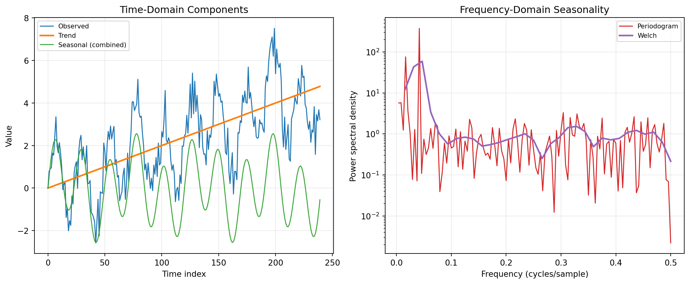
Time-series decomposition separates observed data into interpretable components such as trend, seasonality, and residual variation. In practice, decomposition and seasonality analysis helps analysts distinguish structural change from recurring calendar effects before modeling or forecasting. This distinction matters in operations, finance, and engineering because decisions depend on whether movement is persistent, seasonal, or noise-driven. The same category also connects naturally to frequency-domain methods that reveal periodic structure from power spectra.
The shared concepts are additive/multiplicative structure, trend removal, and periodic energy estimation. Many workflows start from a representation such as y_t = T_t + S_t + R_t (or a multi-seasonal extension), where T_t is trend, S_t is seasonal behavior, and R_t is remainder. Detrending and decomposition operate in the time domain, while spectral estimators quantify how variance is distributed across frequencies. Together, these views provide complementary diagnostics for identifying cycles, validating preprocessing choices, and selecting model assumptions.
Implementation in this category primarily uses statsmodels for decomposition and SciPy Signal for detrending and spectral estimation. Statsmodels provides classical and LOESS-based seasonal decomposition methods for univariate series, while SciPy provides robust signal-processing primitives such as periodograms and Welch PSD estimates. The combined stack is widely used for production analytics because it is transparent, reproducible, and well documented.
For component extraction in the time domain, SEASDECOMP, STL, and MSTL provide progressively more flexible decomposition strategies. SEASDECOMP wraps classical moving-average decomposition and is often used as a baseline when a single stable seasonal period is known. STL performs seasonal-trend decomposition with LOESS smoothing, which is effective when seasonality evolves gradually and robustness to outliers is needed. MSTL extends this idea to multiple seasonalities (for example, intra-week and annual patterns), making it especially useful for high-frequency operational data.
For preprocessing and frequency-domain diagnostics, DETREND, PERIODOGRAM, and WELCH are complementary. DETREND removes constant or linear drift so downstream decomposition and spectral estimates focus on cyclical content rather than low-frequency bias. PERIODOGRAM provides a direct power spectral density estimate and is useful for quickly spotting dominant periodicities. WELCH estimates spectral density by averaging segment periodograms, reducing variance and improving stability when analysts need more reliable peak comparison in noisy signals.
DETREND
This function removes either a linear trend or a constant mean from data along a selected axis. It is commonly used as a preprocessing step before decomposition or spectral analysis.
For constant detrending, the transformed data is:
y_t = x_t - \bar{x}
For linear detrending, the best-fit line a t + b is estimated by least squares and subtracted:
y_t = x_t - (a t + b)
The function returns the detrended data as a rectangular 2D array.
Excel Usage
=DETREND(data, axis, detrend_type, breakpoint, overwrite_data)data(list[list], required): 2D range of numeric values.axis(int, optional, default: -1): Axis along which detrending is applied.detrend_type(str, optional, default: “linear”): Type of detrending to apply.breakpoint(int, optional, default: 0): Breakpoint index for piecewise linear detrending.overwrite_data(bool, optional, default: false): Allow in-place operation to avoid copying.
Returns (list[list]): 2D array of detrended values.
Example 1: Linear detrend on a row vector
Inputs:
| data | axis | detrend_type | breakpoint | overwrite_data | |||||
|---|---|---|---|---|---|---|---|---|---|
| 1 | 2 | 3 | 4 | 5 | 6 | -1 | linear | 0 | false |
Excel formula:
=DETREND({1,2,3,4,5,6}, -1, "linear", 0, FALSE)Expected output:
| Result | |||||
|---|---|---|---|---|---|
| 0 | 2.22045e-16 | 4.44089e-16 | 8.88178e-16 | 8.88178e-16 | 1.77636e-15 |
Example 2: Constant detrend on a row vector
Inputs:
| data | axis | detrend_type | breakpoint | overwrite_data | ||||
|---|---|---|---|---|---|---|---|---|
| 3 | 4 | 5 | 6 | 7 | -1 | constant | 0 | false |
Excel formula:
=DETREND({3,4,5,6,7}, -1, "constant", 0, FALSE)Expected output:
| Result | ||||
|---|---|---|---|---|
| -2 | -1 | 0 | 1 | 2 |
Example 3: Linear detrend across rows in a matrix
Inputs:
| data | axis | detrend_type | breakpoint | overwrite_data | |||
|---|---|---|---|---|---|---|---|
| 1 | 2 | 3 | 4 | 1 | linear | 0 | false |
| 2 | 4 | 6 | 8 |
Excel formula:
=DETREND({1,2,3,4;2,4,6,8}, 1, "linear", 0, FALSE)Expected output:
| Result | |||
|---|---|---|---|
| 7.77156e-16 | 2.22045e-16 | 0 | -8.88178e-16 |
| 1.55431e-15 | 4.44089e-16 | 0 | -1.77636e-15 |
Example 4: Constant detrend along axis zero
Inputs:
| data | axis | detrend_type | breakpoint | overwrite_data | ||
|---|---|---|---|---|---|---|
| 1 | 2 | 3 | 0 | constant | 0 | false |
| 4 | 5 | 6 | ||||
| 7 | 8 | 9 |
Excel formula:
=DETREND({1,2,3;4,5,6;7,8,9}, 0, "constant", 0, FALSE)Expected output:
| Result | ||
|---|---|---|
| -3 | -3 | -3 |
| 0 | 0 | 0 |
| 3 | 3 | 3 |
Python Code
Show Code
import numpy as np
from scipy.signal import detrend as scipy_detrend

def detrend(data, axis=-1, detrend_type='linear', breakpoint=0, overwrite_data=False):
    """
    Remove linear or constant trend from input data.

    See: https://docs.scipy.org/doc/scipy/reference/generated/scipy.signal.detrend.html

    This example function is provided as-is without any representation of accuracy.

    Args:
        data (list[list]): 2D range of numeric values.
        axis (int, optional): Axis along which detrending is applied. Default is -1.
        detrend_type (str, optional): Type of detrending to apply. Valid options: Linear, Constant. Default is 'linear'.
        breakpoint (int, optional): Breakpoint index for piecewise linear detrending. Default is 0.
        overwrite_data (bool, optional): Allow in-place operation to avoid copying. Default is False.

    Returns:
        list[list]: 2D array of detrended values.
    """
    try:
        def to2d(x):
            return [[x]] if not isinstance(x, list) else x

        data = to2d(data)

        if detrend_type not in ("linear", "constant"):
            return "Error: detrend_type must be 'linear' or 'constant'"
        if not isinstance(data, list) or not all(isinstance(row, list) for row in data):
            return "Error: data must be a 2D list"

        matrix = []
        width = None
        for row in data:
            numeric_row = []
            for item in row:
                try:
                    numeric_row.append(float(item))
                except (TypeError, ValueError):
                    return "Error: data must contain only numeric values"

            if width is None:
                width = len(numeric_row)
            elif len(numeric_row) != width:
                return "Error: data must be rectangular"

            matrix.append(numeric_row)

        if not matrix or width == 0:
            return "Error: data must contain at least one numeric value"

        arr = np.asarray(matrix, dtype=float)
        detrended = scipy_detrend(
            arr,
            axis=axis,
            type=detrend_type,
            bp=breakpoint,
            overwrite_data=overwrite_data,
        )

        out = np.asarray(detrended)
        if out.ndim == 1:
            return [[float(v)] for v in out]

        return [[float(v) for v in row] for row in out]
    except Exception as e:
        return f"Error: {str(e)}"
Online Calculator
2D range of numeric values.
Axis along which detrending is applied.
Type of detrending to apply.
Breakpoint index for piecewise linear detrending.
Allow in-place operation to avoid copying.
MSTL
This function applies MSTL to decompose a univariate series that contains multiple seasonal cycles. It estimates trend, one or more seasonal components, and residuals.
The additive structure is:
y_t = T_t + \sum_{k=1}^{K} S_{k,t} + R_t
where K is the number of seasonal periods, S_{k,t} are seasonal components for each period, and R_t is the remainder.
Excel Usage
=MSTL(data, periods, iterate)data(list[list], required): 2D range of time-series values (numeric).periods(list[list], required): 2D range containing one or more seasonal periods (integers greater than 1).iterate(int, optional, default: 2): Number of seasonal refinement iterations.
Returns (list[list]): 2D array with columns [observed, trend, seasonal_1, seasonal_2, …, residual].
Example 1: MSTL with two seasonal periods
Inputs:
| data | periods | iterate | ||||||||||||||||||||
|---|---|---|---|---|---|---|---|---|---|---|---|---|---|---|---|---|---|---|---|---|---|---|
| 20 | 23 | 25 | 22 | 21 | 24 | 26 | 23 | 22 | 25 | 27 | 24 | 23 | 26 | 28 | 25 | 24 | 27 | 29 | 26 | 5 | 10 | 2 |
Excel formula:
=MSTL({20,23,25,22,21,24,26,23,22,25,27,24,23,26,28,25,24,27,29,26}, {5,10}, 2)Expected output:
| Result | |||
|---|---|---|---|
| 20 | 20.4097 | 0.175905 | -0.585603 |
| 23 | 21.2111 | 2.53366 | -0.744755 |
| 25 | 21.9609 | 1.54314 | 1.49601 |
| 22 | 22.7023 | -1.86878 | 1.16644 |
| 21 | 23.4191 | -1.42007 | -0.999054 |
| 24 | 23.485 | 0.313025 | 0.202007 |
| 26 | 23.4437 | 1.02142 | 1.53483 |
| 23 | 23.7658 | 0.537191 | -1.30298 |
| 22 | 24.1849 | -0.564484 | -1.62041 |
| 25 | 24.406 | -0.314793 | 0.908841 |
| 27 | 24.6271 | 0.299052 | 2.07383 |
| 24 | 24.9503 | -0.517282 | -0.433033 |
| 23 | 25.1493 | -0.241955 | -1.90738 |
| 26 | 25.1839 | 0.840148 | -0.024089 |
| 28 | 25.5151 | 0.621596 | 1.86333 |
| 25 | 26.1069 | 0.184459 | -1.29136 |
| 24 | 26.182 | -2.13384 | -0.0481108 |
| 27 | 26.1107 | -0.812054 | 1.7014 |
| 29 | 26.0411 | 2.38302 | 0.57587 |
| 26 | 25.9418 | 1.40994 | -1.35174 |
Example 2: MSTL with a single seasonal period
Inputs:
| data | periods | iterate | |||||||||||
|---|---|---|---|---|---|---|---|---|---|---|---|---|---|
| 10 | 12 | 14 | 12 | 11 | 13 | 15 | 13 | 12 | 14 | 16 | 14 | 4 | 2 |
Excel formula:
=MSTL({10,12,14,12,11,13,15,13,12,14,16,14}, {4}, 2)Expected output:
| Result | |||
|---|---|---|---|
| 10 | 11.625 | -1.625 | 5.32907e-15 |
| 12 | 11.875 | 0.125 | 3.55271e-15 |
| 14 | 12.125 | 1.875 | 1.77636e-15 |
| 12 | 12.375 | -0.375 | 5.32907e-15 |
| 11 | 12.625 | -1.625 | -1.77636e-15 |
| 13 | 12.875 | 0.125 | 0 |
| 15 | 13.125 | 1.875 | 3.55271e-15 |
| 13 | 13.375 | -0.375 | -3.55271e-15 |
| 12 | 13.625 | -1.625 | 0 |
| 14 | 13.875 | 0.125 | 1.77636e-15 |
| 16 | 14.125 | 1.875 | 0 |
| 14 | 14.375 | -0.375 | 3.55271e-15 |
Example 3: MSTL with column-oriented input
Inputs:
| data | periods | iterate |
|---|---|---|
| 10 | 4 | 2 |
| 12 | ||
| 14 | ||
| 12 | ||
| 11 | ||
| 13 | ||
| 15 | ||
| 13 | ||
| 12 | ||
| 14 | ||
| 16 | ||
| 14 |
Excel formula:
=MSTL({10;12;14;12;11;13;15;13;12;14;16;14}, {4}, 2)Expected output:
| Result | |||
|---|---|---|---|
| 10 | 11.625 | -1.625 | 5.32907e-15 |
| 12 | 11.875 | 0.125 | 3.55271e-15 |
| 14 | 12.125 | 1.875 | 1.77636e-15 |
| 12 | 12.375 | -0.375 | 5.32907e-15 |
| 11 | 12.625 | -1.625 | -1.77636e-15 |
| 13 | 12.875 | 0.125 | 0 |
| 15 | 13.125 | 1.875 | 3.55271e-15 |
| 13 | 13.375 | -0.375 | -3.55271e-15 |
| 12 | 13.625 | -1.625 | 0 |
| 14 | 13.875 | 0.125 | 1.77636e-15 |
| 16 | 14.125 | 1.875 | 0 |
| 14 | 14.375 | -0.375 | 3.55271e-15 |
Example 4: MSTL with additional refinement iterations
Inputs:
| data | periods | iterate | ||||||||||||||||||||
|---|---|---|---|---|---|---|---|---|---|---|---|---|---|---|---|---|---|---|---|---|---|---|
| 20 | 23 | 25 | 22 | 21 | 24 | 26 | 23 | 22 | 25 | 27 | 24 | 23 | 26 | 28 | 25 | 24 | 27 | 29 | 26 | 5 | 10 | 3 |
Excel formula:
=MSTL({20,23,25,22,21,24,26,23,22,25,27,24,23,26,28,25,24,27,29,26}, {5,10}, 3)Expected output:
| Result | |||
|---|---|---|---|
| 20 | 20.4097 | 0.175905 | -0.585603 |
| 23 | 21.2111 | 2.53366 | -0.744755 |
| 25 | 21.9609 | 1.54314 | 1.49601 |
| 22 | 22.7023 | -1.86878 | 1.16644 |
| 21 | 23.4191 | -1.42007 | -0.999054 |
| 24 | 23.485 | 0.313025 | 0.202007 |
| 26 | 23.4437 | 1.02142 | 1.53483 |
| 23 | 23.7658 | 0.537191 | -1.30298 |
| 22 | 24.1849 | -0.564484 | -1.62041 |
| 25 | 24.406 | -0.314793 | 0.908841 |
| 27 | 24.6271 | 0.299052 | 2.07383 |
| 24 | 24.9503 | -0.517282 | -0.433033 |
| 23 | 25.1493 | -0.241955 | -1.90738 |
| 26 | 25.1839 | 0.840148 | -0.024089 |
| 28 | 25.5151 | 0.621596 | 1.86333 |
| 25 | 26.1069 | 0.184459 | -1.29136 |
| 24 | 26.182 | -2.13384 | -0.0481108 |
| 27 | 26.1107 | -0.812054 | 1.7014 |
| 29 | 26.0411 | 2.38302 | 0.57587 |
| 26 | 25.9418 | 1.40994 | -1.35174 |
Python Code
Show Code
import numpy as np
from statsmodels.tsa.seasonal import MSTL as sm_MSTL

def mstl(data, periods, iterate=2):
    """
    Perform multi-seasonal STL decomposition on a time series.

    See: https://www.statsmodels.org/stable/generated/statsmodels.tsa.seasonal.MSTL.html

    This example function is provided as-is without any representation of accuracy.

    Args:
        data (list[list]): 2D range of time-series values (numeric).
        periods (list[list]): 2D range containing one or more seasonal periods (integers greater than 1).
        iterate (int, optional): Number of seasonal refinement iterations. Default is 2.

    Returns:
        list[list]: 2D array with columns [observed, trend, seasonal_1, seasonal_2, ..., residual].
    """
    try:
        def to2d(x):
            return [[x]] if not isinstance(x, list) else x

        data = to2d(data)
        periods = to2d(periods)

        if not isinstance(iterate, int) or iterate < 1:
            return "Error: iterate must be an integer greater than or equal to 1"
        if not isinstance(data, list) or not all(isinstance(row, list) for row in data):
            return "Error: data must be a 2D list"
        if not isinstance(periods, list) or not all(isinstance(row, list) for row in periods):
            return "Error: periods must be a 2D list"

        values = []
        for row in data:
            for item in row:
                try:
                    values.append(float(item))
                except (TypeError, ValueError):
                    continue

        period_values = []
        for row in periods:
            for item in row:
                try:
                    p = int(item)
                    if p > 1:
                        period_values.append(p)
                except (TypeError, ValueError):
                    continue

        if not values:
            return "Error: data must contain at least one numeric value"
        if not period_values:
            return "Error: periods must contain at least one integer greater than 1"
        if len(values) < 2 * max(period_values):
            return "Error: data must contain at least two cycles of the largest period"

        period_arg = period_values[0] if len(period_values) == 1 else period_values
        result = sm_MSTL(values, periods=period_arg, iterate=iterate).fit()

        observed = np.asarray(values)
        trend = np.asarray(result.trend)
        seasonal = np.asarray(result.seasonal)
        resid = np.asarray(result.resid)

        if seasonal.ndim == 1:
            seasonal = seasonal.reshape(-1, 1)

        output = []
        for i in range(len(observed)):
            row = [float(observed[i]) if np.isfinite(observed[i]) else ""]
            row.append(float(trend[i]) if np.isfinite(trend[i]) else "")

            for j in range(seasonal.shape[1]):
                val = seasonal[i, j]
                row.append(float(val) if np.isfinite(val) else "")

            row.append(float(resid[i]) if np.isfinite(resid[i]) else "")
            output.append(row)

        return output
    except Exception as e:
        return f"Error: {str(e)}"
Online Calculator
2D range of time-series values (numeric).
2D range containing one or more seasonal periods (integers greater than 1).
Number of seasonal refinement iterations.
PERIODOGRAM
This function computes a periodogram to estimate how signal power is distributed across frequencies. It returns a two-column array containing frequency and estimated spectral power.
The periodogram is based on the squared magnitude of the discrete Fourier transform (DFT):
P(f) \propto |X(f)|^2
where X(f) is the DFT of the input signal. Depending on scaling, the output represents either power spectral density or power spectrum.
Excel Usage
=PERIODOGRAM(data, fs, window, nfft, detrend, return_onesided, scaling)data(list[list], required): 2D range of time-series samples.fs(float, optional, default: 1): Sampling frequency in hertz (Hz).window(str, optional, default: “boxcar”): Window name applied before FFT.nfft(int, optional, default: null): FFT length; null uses input length.detrend(str, optional, default: “constant”): Detrending method for the signal.return_onesided(bool, optional, default: true): Return one-sided spectrum for real-valued input.scaling(str, optional, default: “density”): Spectral scaling mode.
Returns (list[list]): 2D array with columns [frequency, power].
Example 1: Basic periodogram with defaults
Inputs:
| data | fs | window | nfft | detrend | return_onesided | scaling | |||||||||||||||
|---|---|---|---|---|---|---|---|---|---|---|---|---|---|---|---|---|---|---|---|---|---|
| 0 | 1 | 0 | -1 | 0 | 1 | 0 | -1 | 0 | 1 | 0 | -1 | 0 | 1 | 0 | -1 | 8 | boxcar | constant | true | density |
Excel formula:
=PERIODOGRAM({0,1,0,-1,0,1,0,-1,0,1,0,-1,0,1,0,-1}, 8, "boxcar", , "constant", TRUE, "density")Expected output:
| Result | |
|---|---|
| 0 | 0 |
| 0.5 | 0 |
| 1 | 0 |
| 1.5 | 0 |
| 2 | 1 |
| 2.5 | 0 |
| 3 | 0 |
| 3.5 | 0 |
| 4 | 0 |
Example 2: Periodogram with linear detrending
Inputs:
| data | fs | window | nfft | detrend | return_onesided | scaling | |||||||||||||||
|---|---|---|---|---|---|---|---|---|---|---|---|---|---|---|---|---|---|---|---|---|---|
| 0 | 0.8 | 0.1 | -0.9 | -0.2 | 1.1 | 0.2 | -1 | -0.1 | 0.9 | 0 | -1.1 | 0.1 | 1 | -0.2 | -0.8 | 8 | hann | 32 | linear | true | density |
Excel formula:
=PERIODOGRAM({0,0.8,0.1,-0.9,-0.2,1.1,0.2,-1,-0.1,0.9,0,-1.1,0.1,1,-0.2,-0.8}, 8, "hann", 32, "linear", TRUE, "density")Expected output:
| Result | |
|---|---|
| 0 | 0.000128004 |
| 0.25 | 0.00167162 |
| 0.5 | 0.000885883 |
| 0.75 | 0.000758796 |
| 1 | 0.00260373 |
| 1.25 | 0.00674368 |
| 1.5 | 0.118549 |
| 1.75 | 0.426249 |
| 2 | 0.671639 |
| 2.25 | 0.545337 |
| 2.5 | 0.220244 |
| 2.75 | 0.0313019 |
| 3 | 0.0000948799 |
| 3.25 | 0.00383545 |
| 3.5 | 0.00216765 |
| 3.75 | 0.000520404 |
| 4 | 0.00010619 |
Example 3: Periodogram returning power spectrum without detrending
Inputs:
| data | fs | window | nfft | detrend | return_onesided | scaling | |||||||||||||||
|---|---|---|---|---|---|---|---|---|---|---|---|---|---|---|---|---|---|---|---|---|---|
| 0 | 1 | 0 | -1 | 0 | 1 | 0 | -1 | 0 | 1 | 0 | -1 | 0 | 1 | 0 | -1 | 8 | boxcar | none | true | spectrum |
Excel formula:
=PERIODOGRAM({0,1,0,-1,0,1,0,-1,0,1,0,-1,0,1,0,-1}, 8, "boxcar", , "none", TRUE, "spectrum")Expected output:
| Result | |
|---|---|
| 0 | 0 |
| 0.5 | 0 |
| 1 | 0 |
| 1.5 | 0 |
| 2 | 0.5 |
| 2.5 | 0 |
| 3 | 0 |
| 3.5 | 0 |
| 4 | 0 |
Example 4: Two-sided periodogram output
Inputs:
| data | fs | window | nfft | detrend | return_onesided | scaling | |||||||||||||||
|---|---|---|---|---|---|---|---|---|---|---|---|---|---|---|---|---|---|---|---|---|---|
| 0 | 1 | 0 | -1 | 0 | 1 | 0 | -1 | 0 | 1 | 0 | -1 | 0 | 1 | 0 | -1 | 8 | boxcar | constant | false | density |
Excel formula:
=PERIODOGRAM({0,1,0,-1,0,1,0,-1,0,1,0,-1,0,1,0,-1}, 8, "boxcar", , "constant", FALSE, "density")Expected output:
| Result | |
|---|---|
| 0 | 0 |
| 0.5 | 0 |
| 1 | 0 |
| 1.5 | 0 |
| 2 | 0.5 |
| 2.5 | 0 |
| 3 | 0 |
| 3.5 | 0 |
| -4 | 0 |
| -3.5 | 0 |
| -3 | 0 |
| -2.5 | 0 |
| -2 | 0.5 |
| -1.5 | 0 |
| -1 | 0 |
| -0.5 | 0 |
Python Code
Show Code
import numpy as np
from scipy.signal import periodogram as scipy_periodogram

def periodogram(data, fs=1, window='boxcar', nfft=None, detrend='constant', return_onesided=True, scaling='density'):
    """
    Estimate the power spectral density of a time series using a periodogram.

    See: https://docs.scipy.org/doc/scipy/reference/generated/scipy.signal.periodogram.html

    This example function is provided as-is without any representation of accuracy.

    Args:
        data (list[list]): 2D range of time-series samples.
        fs (float, optional): Sampling frequency in hertz (Hz). Default is 1.
        window (str, optional): Window name applied before FFT. Default is 'boxcar'.
        nfft (int, optional): FFT length; null uses input length. Default is None.
        detrend (str, optional): Detrending method for the signal. Valid options: Constant, Linear, None. Default is 'constant'.
        return_onesided (bool, optional): Return one-sided spectrum for real-valued input. Default is True.
        scaling (str, optional): Spectral scaling mode. Valid options: Density, Spectrum. Default is 'density'.

    Returns:
        list[list]: 2D array with columns [frequency, power].
    """
    try:
        def to2d(x):
            return [[x]] if not isinstance(x, list) else x

        data = to2d(data)

        if fs <= 0:
            return "Error: fs must be greater than 0"
        if detrend not in ("constant", "linear", "none"):
            return "Error: detrend must be 'constant', 'linear', or 'none'"
        if scaling not in ("density", "spectrum"):
            return "Error: scaling must be 'density' or 'spectrum'"
        if not isinstance(data, list) or not all(isinstance(row, list) for row in data):
            return "Error: data must be a 2D list"

        values = []
        for row in data:
            for item in row:
                try:
                    values.append(float(item))
                except (TypeError, ValueError):
                    continue

        if len(values) < 2:
            return "Error: data must contain at least two numeric values"

        nfft_arg = None if nfft is None or nfft <= 0 else nfft
        detrend_arg = False if detrend == "none" else detrend

        freqs, power = scipy_periodogram(
            np.asarray(values, dtype=float),
            fs=fs,
            window=window,
            nfft=nfft_arg,
            detrend=detrend_arg,
            return_onesided=return_onesided,
            scaling=scaling,
        )

        return [[float(freqs[i]), float(power[i])] for i in range(len(freqs))]
    except Exception as e:
        return f"Error: {str(e)}"
Online Calculator
2D range of time-series samples.
Sampling frequency in hertz (Hz).
Window name applied before FFT.
FFT length; null uses input length.
Detrending method for the signal.
Return one-sided spectrum for real-valued input.
Spectral scaling mode.
SEASDECOMP
This function performs classical seasonal decomposition using moving averages. It splits a univariate time series into observed, trend, seasonal, and residual components under either an additive or multiplicative model.
For an additive model, the decomposition is:
y_t = T_t + S_t + R_t
For a multiplicative model, the decomposition is:
y_t = T_t \times S_t \times R_t
The input must contain at least two full seasonal cycles so that seasonal effects can be estimated reliably.
Excel Usage
=SEASDECOMP(data, period, model, two_sided, extrapolate_points)data(list[list], required): 2D range of time-series values (numeric).period(int, required): Seasonal period in samples (positive integer).model(str, optional, default: “additive”): Seasonal decomposition model type.two_sided(bool, optional, default: true): Use centered moving average when true.extrapolate_points(int, optional, default: 0): Number of nearest points used to extrapolate trend at boundaries.
Returns (list[list]): 2D array with columns [observed, trend, seasonal, residual].
Example 1: Additive decomposition with quarterly-style period
Inputs:
| data | period | model | two_sided | extrapolate_points | |||||||||||
|---|---|---|---|---|---|---|---|---|---|---|---|---|---|---|---|
| 10 | 12 | 14 | 12 | 11 | 13 | 15 | 13 | 12 | 14 | 16 | 14 | 4 | additive | true | 0 |
Excel formula:
=SEASDECOMP({10,12,14,12,11,13,15,13,12,14,16,14}, 4, "additive", TRUE, 0)Expected output:
| Result | |||
|---|---|---|---|
| 10 | -1.625 | ||
| 12 | 0.125 | ||
| 14 | 12.125 | 1.875 | 0 |
| 12 | 12.375 | -0.375 | 0 |
| 11 | 12.625 | -1.625 | 0 |
| 13 | 12.875 | 0.125 | 0 |
| 15 | 13.125 | 1.875 | 0 |
| 13 | 13.375 | -0.375 | 0 |
| 12 | 13.625 | -1.625 | 0 |
| 14 | 13.875 | 0.125 | 0 |
| 16 | 1.875 | ||
| 14 | -0.375 |
Example 2: Multiplicative decomposition with positive series
Inputs:
| data | period | model | two_sided | extrapolate_points | |||||||||||
|---|---|---|---|---|---|---|---|---|---|---|---|---|---|---|---|
| 10 | 20 | 15 | 25 | 11 | 22 | 16 | 27 | 12 | 24 | 18 | 30 | 4 | multiplicative | true | 0 |
Excel formula:
=SEASDECOMP({10,20,15,25,11,22,16,27,12,24,18,30}, 4, "multiplicative", TRUE, 0)Expected output:
| Result | |||
|---|---|---|---|
| 10 | 0.599561 | ||
| 20 | 1.16896 | ||
| 15 | 17.625 | 0.844172 | 1.00816 |
| 25 | 18 | 1.38731 | 1.00114 |
| 11 | 18.375 | 0.599561 | 0.998463 |
| 22 | 18.75 | 1.16896 | 1.00375 |
| 16 | 19.125 | 0.844172 | 0.991031 |
| 27 | 19.5 | 1.38731 | 0.998057 |
| 12 | 20 | 0.599561 | 1.00073 |
| 24 | 20.625 | 1.16896 | 0.99545 |
| 18 | 0.844172 | ||
| 30 | 1.38731 |
Example 3: Single-column data is flattened and decomposed
Inputs:
| data | period | model | two_sided | extrapolate_points |
|---|---|---|---|---|
| 10 | 4 | additive | true | 0 |
| 12 | ||||
| 14 | ||||
| 12 | ||||
| 11 | ||||
| 13 | ||||
| 15 | ||||
| 13 | ||||
| 12 | ||||
| 14 | ||||
| 16 | ||||
| 14 |
Excel formula:
=SEASDECOMP({10;12;14;12;11;13;15;13;12;14;16;14}, 4, "additive", TRUE, 0)Expected output:
| Result | |||
|---|---|---|---|
| 10 | -1.625 | ||
| 12 | 0.125 | ||
| 14 | 12.125 | 1.875 | 0 |
| 12 | 12.375 | -0.375 | 0 |
| 11 | 12.625 | -1.625 | 0 |
| 13 | 12.875 | 0.125 | 0 |
| 15 | 13.125 | 1.875 | 0 |
| 13 | 13.375 | -0.375 | 0 |
| 12 | 13.625 | -1.625 | 0 |
| 14 | 13.875 | 0.125 | 0 |
| 16 | 1.875 | ||
| 14 | -0.375 |
Example 4: One-sided moving average decomposition
Inputs:
| data | period | model | two_sided | extrapolate_points | |||||||||||
|---|---|---|---|---|---|---|---|---|---|---|---|---|---|---|---|
| 10 | 12 | 14 | 12 | 11 | 13 | 15 | 13 | 12 | 14 | 16 | 14 | 4 | additive | false | 1 |
Excel formula:
=SEASDECOMP({10,12,14,12,11,13,15,13,12,14,16,14}, 4, "additive", FALSE, 1)Expected output:
| Result | |||
|---|---|---|---|
| 10 | 11.125 | -1.625 | 0.5 |
| 12 | 11.375 | 0.125 | 0.5 |
| 14 | 11.625 | 1.875 | 0.5 |
| 12 | 11.875 | -0.375 | 0.5 |
| 11 | 12.125 | -1.625 | 0.5 |
| 13 | 12.375 | 0.125 | 0.5 |
| 15 | 12.625 | 1.875 | 0.5 |
| 13 | 12.875 | -0.375 | 0.5 |
| 12 | 13.125 | -1.625 | 0.5 |
| 14 | 13.375 | 0.125 | 0.5 |
| 16 | 13.625 | 1.875 | 0.5 |
| 14 | 13.875 | -0.375 | 0.5 |
Python Code
Show Code
import numpy as np
from statsmodels.tsa.seasonal import seasonal_decompose as sm_seasonal_decompose

def seasdecomp(data, period, model='additive', two_sided=True, extrapolate_points=0):
    """
    Decompose a time series into trend, seasonal, and residual components.

    See: https://www.statsmodels.org/stable/generated/statsmodels.tsa.seasonal.seasonal_decompose.html

    This example function is provided as-is without any representation of accuracy.

    Args:
        data (list[list]): 2D range of time-series values (numeric).
        period (int): Seasonal period in samples (positive integer).
        model (str, optional): Seasonal decomposition model type. Valid options: Additive, Multiplicative. Default is 'additive'.
        two_sided (bool, optional): Use centered moving average when true. Default is True.
        extrapolate_points (int, optional): Number of nearest points used to extrapolate trend at boundaries. Default is 0.

    Returns:
        list[list]: 2D array with columns [observed, trend, seasonal, residual].
    """
    try:
        def to2d(x):
            return [[x]] if not isinstance(x, list) else x

        data = to2d(data)

        if model not in ("additive", "multiplicative"):
            return "Error: model must be 'additive' or 'multiplicative'"
        if not isinstance(period, int) or period < 2:
            return "Error: period must be an integer greater than or equal to 2"
        if not isinstance(data, list) or not all(isinstance(row, list) for row in data):
            return "Error: data must be a 2D list"

        values = []
        for row in data:
            for item in row:
                try:
                    values.append(float(item))
                except (TypeError, ValueError):
                    continue

        if len(values) < 2 * period:
            return "Error: data must contain at least two complete seasonal cycles"

        result = sm_seasonal_decompose(
            values,
            model=model,
            period=period,
            two_sided=two_sided,
            extrapolate_trend=extrapolate_points,
        )

        observed = np.asarray(result.observed)
        trend = np.asarray(result.trend)
        seasonal = np.asarray(result.seasonal)
        resid = np.asarray(result.resid)

        output = []
        for i in range(len(observed)):
            row = []
            for arr in (observed, trend, seasonal, resid):
                val = arr[i]
                row.append(float(val) if np.isfinite(val) else "")
            output.append(row)

        return output
    except Exception as e:
        return f"Error: {str(e)}"
Online Calculator
2D range of time-series values (numeric).
Seasonal period in samples (positive integer).
Seasonal decomposition model type.
Use centered moving average when true.
Number of nearest points used to extrapolate trend at boundaries.
STL
This function applies STL (Seasonal-Trend decomposition using LOESS) to a univariate time series and returns observed, trend, seasonal, and residual components.
STL models a series as:
y_t = T_t + S_t + R_t
where T_t is a smooth trend, S_t is a seasonal component with known period, and R_t is the remainder. The robust option can reduce the influence of outliers.
Excel Usage
=STL(data, period, seasonal, robust)data(list[list], required): 2D range of time-series values (numeric).period(int, required): Seasonal period in samples (positive integer).seasonal(int, optional, default: 7): Length of seasonal smoother (odd integer).robust(bool, optional, default: false): Use robust fitting to reduce outlier influence.
Returns (list[list]): 2D array with columns [observed, trend, seasonal, residual].
Example 1: STL decomposition of seasonal series
Inputs:
| data | period | seasonal | robust | |||||||||||||||
|---|---|---|---|---|---|---|---|---|---|---|---|---|---|---|---|---|---|---|
| 10 | 12 | 14 | 12 | 11 | 13 | 15 | 13 | 12 | 14 | 16 | 14 | 13 | 15 | 17 | 15 | 4 | 7 | false |
Excel formula:
=STL({10,12,14,12,11,13,15,13,12,14,16,14,13,15,17,15}, 4, 7, FALSE)Expected output:
| Result | |||
|---|---|---|---|
| 10 | 11.625 | -1.625 | 0 |
| 12 | 11.875 | 0.125 | 1.77636e-15 |
| 14 | 12.125 | 1.875 | 0 |
| 12 | 12.375 | -0.375 | 1.77636e-15 |
| 11 | 12.625 | -1.625 | 0 |
| 13 | 12.875 | 0.125 | -1.77636e-15 |
| 15 | 13.125 | 1.875 | 1.77636e-15 |
| 13 | 13.375 | -0.375 | 1.77636e-15 |
| 12 | 13.625 | -1.625 | 1.77636e-15 |
| 14 | 13.875 | 0.125 | 3.55271e-15 |
| 16 | 14.125 | 1.875 | -5.32907e-15 |
| 14 | 14.375 | -0.375 | 0 |
| 13 | 14.625 | -1.625 | 7.10543e-15 |
| 15 | 14.875 | 0.125 | 3.55271e-15 |
| 17 | 15.125 | 1.875 | 8.88178e-15 |
| 15 | 15.375 | -0.375 | 7.10543e-15 |
Example 2: Robust STL decomposition
Inputs:
| data | period | seasonal | robust | |||||||||||||||
|---|---|---|---|---|---|---|---|---|---|---|---|---|---|---|---|---|---|---|
| 10 | 12 | 14 | 12 | 11 | 13 | 15 | 13 | 12 | 14 | 16 | 14 | 13 | 15 | 17 | 15 | 4 | 7 | true |
Excel formula:
=STL({10,12,14,12,11,13,15,13,12,14,16,14,13,15,17,15}, 4, 7, TRUE)Expected output:
| Result | |||
|---|---|---|---|
| 10 | 11.625 | -1.625 | -7.10543e-15 |
| 12 | 11.875 | 0.125 | 0 |
| 14 | 12.125 | 1.875 | 0 |
| 12 | 12.375 | -0.375 | 1.77636e-15 |
| 11 | 12.625 | -1.625 | 3.55271e-15 |
| 13 | 12.875 | 0.125 | 1.77636e-15 |
| 15 | 13.125 | 1.875 | 0 |
| 13 | 13.375 | -0.375 | -5.32907e-15 |
| 12 | 13.625 | -1.625 | 8.88178e-15 |
| 14 | 13.875 | 0.125 | 1.77636e-15 |
| 16 | 14.125 | 1.875 | -1.77636e-15 |
| 14 | 14.375 | -0.375 | -1.77636e-15 |
| 13 | 14.625 | -1.625 | -1.06581e-14 |
| 15 | 14.875 | 0.125 | -1.95399e-14 |
| 17 | 15.125 | 1.875 | 4.44089e-14 |
| 15 | 15.375 | -0.375 | -8.34888e-14 |
Example 3: STL with single-column range input
Inputs:
| data | period | seasonal | robust |
|---|---|---|---|
| 10 | 4 | 7 | false |
| 12 | |||
| 14 | |||
| 12 | |||
| 11 | |||
| 13 | |||
| 15 | |||
| 13 | |||
| 12 | |||
| 14 | |||
| 16 | |||
| 14 | |||
| 13 | |||
| 15 | |||
| 17 | |||
| 15 |
Excel formula:
=STL({10;12;14;12;11;13;15;13;12;14;16;14;13;15;17;15}, 4, 7, FALSE)Expected output:
| Result | |||
|---|---|---|---|
| 10 | 11.625 | -1.625 | 0 |
| 12 | 11.875 | 0.125 | 1.77636e-15 |
| 14 | 12.125 | 1.875 | 0 |
| 12 | 12.375 | -0.375 | 1.77636e-15 |
| 11 | 12.625 | -1.625 | 0 |
| 13 | 12.875 | 0.125 | -1.77636e-15 |
| 15 | 13.125 | 1.875 | 1.77636e-15 |
| 13 | 13.375 | -0.375 | 1.77636e-15 |
| 12 | 13.625 | -1.625 | 1.77636e-15 |
| 14 | 13.875 | 0.125 | 3.55271e-15 |
| 16 | 14.125 | 1.875 | -5.32907e-15 |
| 14 | 14.375 | -0.375 | 0 |
| 13 | 14.625 | -1.625 | 7.10543e-15 |
| 15 | 14.875 | 0.125 | 3.55271e-15 |
| 17 | 15.125 | 1.875 | 8.88178e-15 |
| 15 | 15.375 | -0.375 | 7.10543e-15 |
Example 4: STL with longer period and data length
Inputs:
| data | period | seasonal | robust | |||||||||||||||||||||||
|---|---|---|---|---|---|---|---|---|---|---|---|---|---|---|---|---|---|---|---|---|---|---|---|---|---|---|
| 20 | 21 | 23 | 25 | 24 | 22 | 21 | 22 | 24 | 26 | 25 | 23 | 22 | 23 | 25 | 27 | 26 | 24 | 23 | 24 | 26 | 28 | 27 | 25 | 6 | 7 | false |
Excel formula:
=STL({20,21,23,25,24,22,21,22,24,26,25,23,22,23,25,27,26,24,23,24,26,28,27,25}, 6, 7, FALSE)Expected output:
| Result | |||
|---|---|---|---|
| 20 | 22.0833 | -2.08333 | 0 |
| 21 | 22.25 | -1.25 | 7.10543e-15 |
| 23 | 22.4167 | 0.583333 | 3.55271e-15 |
| 25 | 22.5833 | 2.41667 | 3.55271e-15 |
| 24 | 22.75 | 1.25 | 3.55271e-15 |
| 22 | 22.9167 | -0.916667 | -3.55271e-15 |
| 21 | 23.0833 | -2.08333 | 3.55271e-15 |
| 22 | 23.25 | -1.25 | -7.10543e-15 |
| 24 | 23.4167 | 0.583333 | -3.55271e-15 |
| 26 | 23.5833 | 2.41667 | -3.55271e-15 |
| 25 | 23.75 | 1.25 | -3.55271e-15 |
| 23 | 23.9167 | -0.916667 | 3.55271e-15 |
| 22 | 24.0833 | -2.08333 | -3.55271e-15 |
| 23 | 24.25 | -1.25 | 0 |
| 25 | 24.4167 | 0.583333 | 3.55271e-15 |
| 27 | 24.5833 | 2.41667 | 3.55271e-15 |
| 26 | 24.75 | 1.25 | -7.10543e-15 |
| 24 | 24.9167 | -0.916667 | 3.55271e-15 |
| 23 | 25.0833 | -2.08333 | -3.55271e-15 |
| 24 | 25.25 | -1.25 | 0 |
| 26 | 25.4167 | 0.583333 | -1.06581e-14 |
| 28 | 25.5833 | 2.41667 | -1.06581e-14 |
| 27 | 25.75 | 1.25 | -3.55271e-15 |
| 25 | 25.9167 | -0.916667 | -1.06581e-14 |
Python Code
Show Code
import numpy as np
from statsmodels.tsa.seasonal import STL as sm_STL

def stl(data, period, seasonal=7, robust=False):
    """
    Perform STL decomposition of a univariate time series.

    See: https://www.statsmodels.org/stable/generated/statsmodels.tsa.seasonal.STL.html

    This example function is provided as-is without any representation of accuracy.

    Args:
        data (list[list]): 2D range of time-series values (numeric).
        period (int): Seasonal period in samples (positive integer).
        seasonal (int, optional): Length of seasonal smoother (odd integer). Default is 7.
        robust (bool, optional): Use robust fitting to reduce outlier influence. Default is False.

    Returns:
        list[list]: 2D array with columns [observed, trend, seasonal, residual].
    """
    try:
        def to2d(x):
            return [[x]] if not isinstance(x, list) else x

        data = to2d(data)

        if not isinstance(period, int) or period < 2:
            return "Error: period must be an integer greater than or equal to 2"
        if not isinstance(seasonal, int) or seasonal < 3 or seasonal % 2 == 0:
            return "Error: seasonal must be an odd integer greater than or equal to 3"
        if not isinstance(data, list) or not all(isinstance(row, list) for row in data):
            return "Error: data must be a 2D list"

        values = []
        for row in data:
            for item in row:
                try:
                    values.append(float(item))
                except (TypeError, ValueError):
                    continue

        if len(values) < 2 * period:
            return "Error: data must contain at least two complete seasonal cycles"

        result = sm_STL(values, period=period, seasonal=seasonal, robust=robust).fit()

        observed = np.asarray(values)
        trend = np.asarray(result.trend)
        seasonal_comp = np.asarray(result.seasonal)
        resid = np.asarray(result.resid)

        output = []
        for i in range(len(observed)):
            row = []
            for arr in (observed, trend, seasonal_comp, resid):
                val = arr[i]
                row.append(float(val) if np.isfinite(val) else "")
            output.append(row)

        return output
    except Exception as e:
        return f"Error: {str(e)}"
Online Calculator
2D range of time-series values (numeric).
Seasonal period in samples (positive integer).
Length of seasonal smoother (odd integer).
Use robust fitting to reduce outlier influence.
WELCH
This function computes Welch’s spectral density estimate by splitting a signal into overlapping segments, computing a modified periodogram for each segment, and averaging the results.
Compared with a simple periodogram, Welch’s method reduces variance in spectral estimates by averaging across segments.
If segment periodograms are P_1(f), \dots, P_m(f), Welch estimates:
\hat{P}(f) = \frac{1}{m} \sum_{i=1}^{m} P_i(f)
or a median-based alternative when median averaging is selected.
Excel Usage
=WELCH(data, fs, window, nperseg, noverlap, nfft, detrend, return_onesided, scaling, average)data(list[list], required): 2D range of time-series samples.fs(float, optional, default: 1): Sampling frequency in hertz (Hz).window(str, optional, default: “hann”): Window name applied to each segment.nperseg(int, optional, default: null): Segment length; null uses SciPy default.noverlap(int, optional, default: null): Overlap length between adjacent segments; null uses default.nfft(int, optional, default: null): FFT length; null uses segment length.detrend(str, optional, default: “constant”): Detrending method applied per segment.return_onesided(bool, optional, default: true): Return one-sided spectrum for real-valued input.scaling(str, optional, default: “density”): Spectral scaling mode.average(str, optional, default: “mean”): Averaging method across segment periodograms.
Returns (list[list]): 2D array with columns [frequency, power].
Example 1: Welch PSD with default averaging
Inputs:
| data | fs | window | nperseg | noverlap | nfft | detrend | return_onesided | scaling | average | |||||||||||||||
|---|---|---|---|---|---|---|---|---|---|---|---|---|---|---|---|---|---|---|---|---|---|---|---|---|
| 0 | 1 | 0 | -1 | 0 | 1 | 0 | -1 | 0 | 1 | 0 | -1 | 0 | 1 | 0 | -1 | 8 | hann | 8 | 4 | constant | true | density | mean |
Excel formula:
=WELCH({0,1,0,-1,0,1,0,-1,0,1,0,-1,0,1,0,-1}, 8, "hann", 8, 4, , "constant", TRUE, "density", "mean")Expected output:
| Result | |
|---|---|
| 0 | 0 |
| 1 | 0.0833333 |
| 2 | 0.333333 |
| 3 | 0.0833333 |
| 4 | 0 |
Example 2: Welch PSD with median averaging
Inputs:
| data | fs | window | nperseg | noverlap | nfft | detrend | return_onesided | scaling | average | |||||||||||||||
|---|---|---|---|---|---|---|---|---|---|---|---|---|---|---|---|---|---|---|---|---|---|---|---|---|
| 0 | 0.8 | 0.1 | -0.9 | -0.2 | 1.1 | 0.2 | -1 | -0.1 | 0.9 | 0 | -1.1 | 0.1 | 1 | -0.2 | -0.8 | 8 | hann | 8 | 4 | 16 | constant | true | density | median |
Excel formula:
=WELCH({0,0.8,0.1,-0.9,-0.2,1.1,0.2,-1,-0.1,0.9,0,-1.1,0.1,1,-0.2,-0.8}, 8, "hann", 8, 4, 16, "constant", TRUE, "density", "median")Expected output:
| Result | |
|---|---|
| 0 | 0.0000428932 |
| 0.5 | 0.0150076 |
| 1 | 0.0989203 |
| 1.5 | 0.284435 |
| 2 | 0.40062 |
| 2.5 | 0.288359 |
| 3 | 0.105885 |
| 3.5 | 0.0198086 |
| 4 | 0.000364277 |
Example 3: Welch with linear detrending
Inputs:
| data | fs | window | nperseg | noverlap | nfft | detrend | return_onesided | scaling | average | |||||||||||||||
|---|---|---|---|---|---|---|---|---|---|---|---|---|---|---|---|---|---|---|---|---|---|---|---|---|
| 0 | 0.8 | 0.1 | -0.9 | -0.2 | 1.1 | 0.2 | -1 | -0.1 | 0.9 | 0 | -1.1 | 0.1 | 1 | -0.2 | -0.8 | 8 | hann | 8 | 2 | linear | true | density | mean |
Excel formula:
=WELCH({0,0.8,0.1,-0.9,-0.2,1.1,0.2,-1,-0.1,0.9,0,-1.1,0.1,1,-0.2,-0.8}, 8, "hann", 8, 2, , "linear", TRUE, "density", "mean")Expected output:
| Result | |
|---|---|
| 0 | 0.00320211 |
| 1 | 0.141449 |
| 2 | 0.356001 |
| 3 | 0.0927694 |
| 4 | 0.00137051 |
Example 4: Two-sided Welch power spectrum
Inputs:
| data | fs | window | nperseg | noverlap | nfft | detrend | return_onesided | scaling | average | |||||||||||||||
|---|---|---|---|---|---|---|---|---|---|---|---|---|---|---|---|---|---|---|---|---|---|---|---|---|
| 0 | 1 | 0 | -1 | 0 | 1 | 0 | -1 | 0 | 1 | 0 | -1 | 0 | 1 | 0 | -1 | 8 | hann | 8 | 4 | none | false | spectrum | mean |
Excel formula:
=WELCH({0,1,0,-1,0,1,0,-1,0,1,0,-1,0,1,0,-1}, 8, "hann", 8, 4, , "none", FALSE, "spectrum", "mean")Expected output:
| Result | |
|---|---|
| 0 | 0 |
| 1 | 0.0625 |
| 2 | 0.25 |
| 3 | 0.0625 |
| -4 | 0 |
| -3 | 0.0625 |
| -2 | 0.25 |
| -1 | 0.0625 |
Python Code
Show Code
import numpy as np
from scipy.signal import welch as scipy_welch

def welch(data, fs=1, window='hann', nperseg=None, noverlap=None, nfft=None, detrend='constant', return_onesided=True, scaling='density', average='mean'):
    """
    Estimate the power spectral density of a time series using Welch's method.

    See: https://docs.scipy.org/doc/scipy/reference/generated/scipy.signal.welch.html

    This example function is provided as-is without any representation of accuracy.

    Args:
        data (list[list]): 2D range of time-series samples.
        fs (float, optional): Sampling frequency in hertz (Hz). Default is 1.
        window (str, optional): Window name applied to each segment. Default is 'hann'.
        nperseg (int, optional): Segment length; null uses SciPy default. Default is None.
        noverlap (int, optional): Overlap length between adjacent segments; null uses default. Default is None.
        nfft (int, optional): FFT length; null uses segment length. Default is None.
        detrend (str, optional): Detrending method applied per segment. Valid options: Constant, Linear, None. Default is 'constant'.
        return_onesided (bool, optional): Return one-sided spectrum for real-valued input. Default is True.
        scaling (str, optional): Spectral scaling mode. Valid options: Density, Spectrum. Default is 'density'.
        average (str, optional): Averaging method across segment periodograms. Valid options: Mean, Median. Default is 'mean'.

    Returns:
        list[list]: 2D array with columns [frequency, power].
    """
    try:
        def to2d(x):
            return [[x]] if not isinstance(x, list) else x

        data = to2d(data)

        if fs <= 0:
            return "Error: fs must be greater than 0"
        if detrend not in ("constant", "linear", "none"):
            return "Error: detrend must be 'constant', 'linear', or 'none'"
        if scaling not in ("density", "spectrum"):
            return "Error: scaling must be 'density' or 'spectrum'"
        if average not in ("mean", "median"):
            return "Error: average must be 'mean' or 'median'"
        if not isinstance(data, list) or not all(isinstance(row, list) for row in data):
            return "Error: data must be a 2D list"

        values = []
        for row in data:
            for item in row:
                try:
                    values.append(float(item))
                except (TypeError, ValueError):
                    continue

        if len(values) < 2:
            return "Error: data must contain at least two numeric values"

        nperseg_arg = None if nperseg is None or nperseg <= 0 else nperseg
        noverlap_arg = None if noverlap is None or noverlap < 0 else noverlap
        nfft_arg = None if nfft is None or nfft <= 0 else nfft
        detrend_arg = False if detrend == "none" else detrend

        if nperseg_arg is not None and noverlap_arg is not None and noverlap_arg >= nperseg_arg:
            return "Error: noverlap must be smaller than nperseg"

        freqs, power = scipy_welch(
            np.asarray(values, dtype=float),
            fs=fs,
            window=window,
            nperseg=nperseg_arg,
            noverlap=noverlap_arg,
            nfft=nfft_arg,
            detrend=detrend_arg,
            return_onesided=return_onesided,
            scaling=scaling,
            average=average,
        )

        return [[float(freqs[i]), float(power[i])] for i in range(len(freqs))]
    except Exception as e:
        return f"Error: {str(e)}"
Online Calculator
2D range of time-series samples.
Sampling frequency in hertz (Hz).
Window name applied to each segment.
Segment length; null uses SciPy default.
Overlap length between adjacent segments; null uses default.
FFT length; null uses segment length.
Detrending method applied per segment.
Return one-sided spectrum for real-valued input.
Spectral scaling mode.
Averaging method across segment periodograms.