Overview
Calculus is the mathematical study of continuous change, providing the theoretical foundation for modeling dynamic systems across science, engineering, and economics. The two fundamental operations—differentiation (measuring rates of change) and integration (computing accumulated quantities)—enable us to analyze everything from population growth and chemical reactions to planetary motion and market dynamics. When combined with ordinary differential equations (ODEs), calculus becomes a powerful tool for predicting system behavior over time.
In physics and engineering, calculus describes motion, heat transfer, fluid dynamics, and electrical circuits. In biology and medicine, it models population dynamics, epidemics, and pharmacokinetics. In economics and finance, it underpins optimal control theory, option pricing, and growth models. The tools in this category bring these computational capabilities directly into Excel, leveraging Python’s SciPy and CasADi libraries for numerical and symbolic computation.
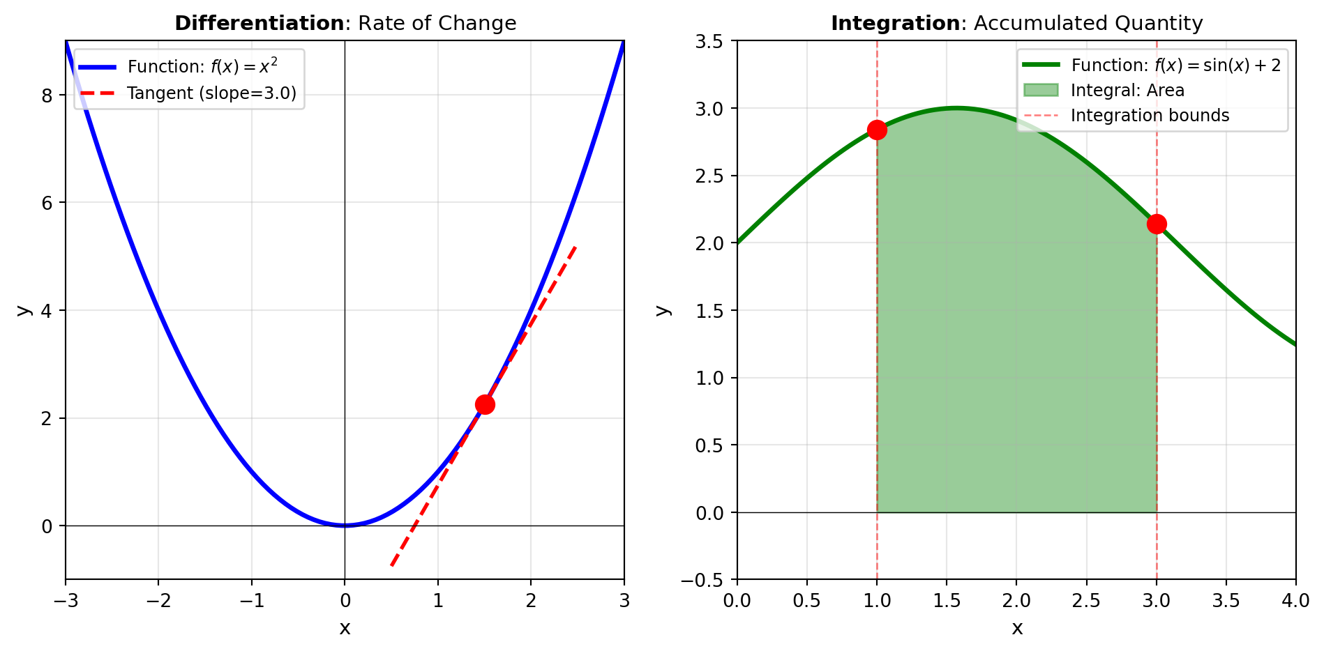
Differentiation encompasses computing derivatives of functions—from simple univariate derivatives to structured approaches like the Jacobian matrix (first-order partial derivatives of vector-valued functions) and the Hessian matrix (second-order partial derivatives for optimization). Tools like JACOBIAN and HESSIAN enable sensitivity analysis and optimization support, while SENSITIVITY directly computes parameter sensitivities for model outputs.
Integration computes accumulated quantities, from evaluating definite integrals of smooth functions to integrating sampled data. Tools like QUAD and DBLQUAD perform numerical integration over one and two dimensions, while TRAPEZOID applies the composite trapezoidal rule to discrete datasets.
ODE models and solvers form the core of dynamical system simulation. Predefined models—LORENZ, LOTKA_VOLTERRA, SIR, SEIR—demonstrate canonical systems in chaos, ecology, and epidemiology. General solvers SOLVE_IVP and SOLVE_BVP handle arbitrary initial value and boundary value problems, enabling custom model definitions.
<>:36: SyntaxWarning: invalid escape sequence '\s'
<>:36: SyntaxWarning: invalid escape sequence '\s'
/tmp/ipykernel_73105/3400740372.py:36: SyntaxWarning: invalid escape sequence '\s'
  ax2.plot(x2, y2, 'g-', linewidth=2.5, label='Function: $f(x) = \sin(x) + 2$')
Differentiation
| HESSIAN |
Compute the Hessian matrix (second derivatives) of a scalar function using CasADi symbolic differentiation. |
| JACOBIAN |
Calculate the Jacobian matrix of mathematical expressions with respect to specified variables. |
| SENSITIVITY |
Compute the sensitivity of a scalar model with respect to its parameters using CasADi. |
Integration
| DBLQUAD |
Compute the double integral of a function over a two-dimensional region. |
| QUAD |
Numerically integrate a function defined by a table of x, y values over [a, b] using adaptive quadrature. |
| TRAPEZOID |
Integrate sampled data using the composite trapezoidal rule. |
Ode Models
| BRUSSELATOR |
Numerically solves the Brusselator system of ordinary differential equations for autocatalytic chemical reactions. |
| COMPARTMENTAL_PK |
Numerically solves the basic one-compartment pharmacokinetics ODE using scipy.integrate.solve_ivp. |
| FITZHUGH_NAGUMO |
Numerically solves the FitzHugh-Nagumo system of ordinary differential equations for neuron action potentials using scipy.integrate.solve_ivp. |
| HODGKIN_HUXLEY |
Numerically solves the Hodgkin-Huxley system of ordinary differential equations for neuron action potentials. |
| LORENZ |
Numerically solves the Lorenz system of ordinary differential equations for chaotic dynamics. |
| LOTKA_VOLTERRA |
Numerically solves the Lotka-Volterra predator-prey system of ordinary differential equations. |
| MICHAELIS_MENTEN |
Numerically solves the Michaelis-Menten system of ordinary differential equations for enzyme kinetics using scipy.integrate.solve_ivp. |
| SEIR |
Numerically solves the SEIR system of ordinary differential equations for infectious disease modeling using scipy.integrate.solve_ivp. |
| SIR |
Solves the SIR system of ordinary differential equations for infection dynamics using scipy.integrate.solve_ivp (see scipy.integrate.solve_ivp). |
| VAN_DER_POL |
Numerically solves the Van der Pol oscillator system of ordinary differential equations. |
Ode Systems
| SOLVE_BVP |
Solve a boundary value problem for a second-order system of ODEs. |
| SOLVE_IVP |
Solve an initial value problem for a system of ODEs of the form dy/dt = A @ y. |