Models
Overview
Curve fitting is the process of constructing a mathematical function that best describes the relationship between independent and dependent variables in experimental or observational data. While general-purpose regression techniques can approximate any smooth relationship, domain-specific models encode physical laws, chemical kinetics, biological mechanisms, or engineering principles directly into the functional form. This approach reduces the number of free parameters, improves interpretability, and often yields more reliable extrapolation beyond the measured range.
Why Domain-Specific Models Matter
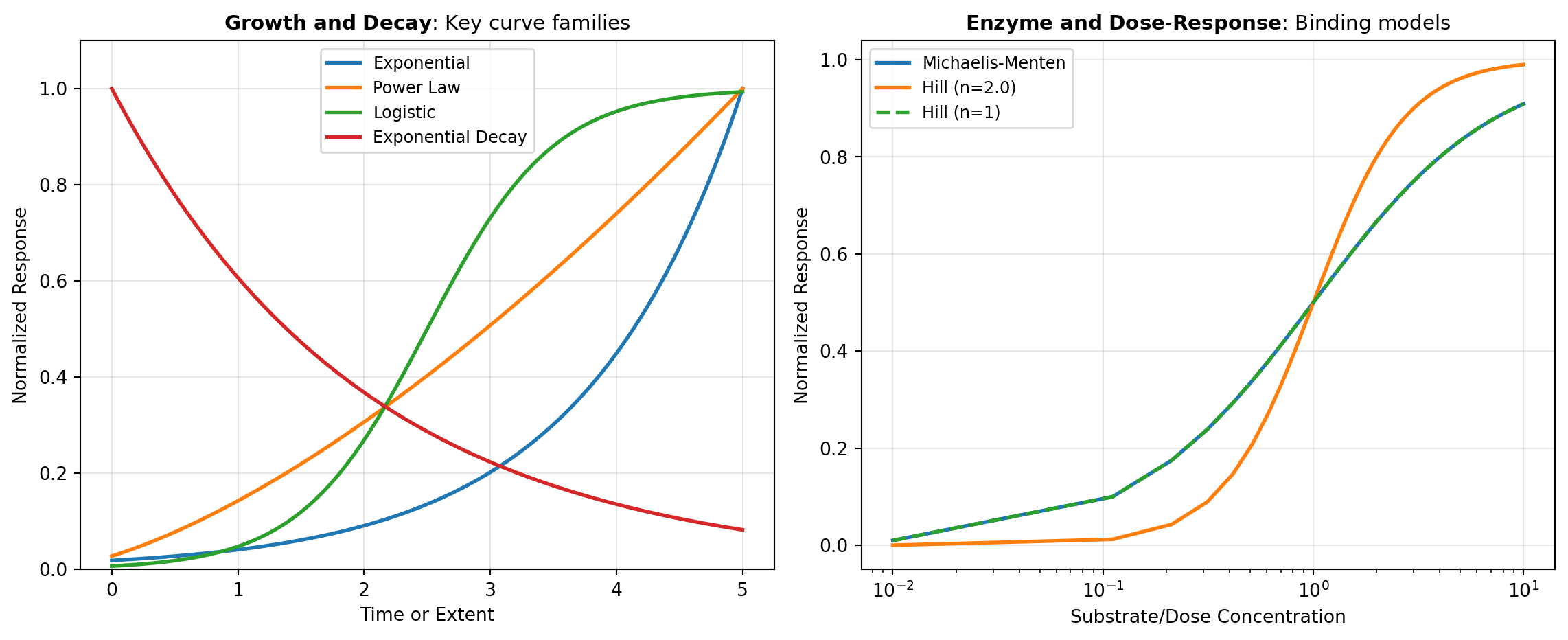
The power of domain-specific modeling lies in leveraging domain knowledge to inform the functional form of your model. Rather than fitting a generic polynomial or spline that might adapt to noise, a model based on underlying physics or chemistry captures the true mechanism generating your data. For example, exponential growth in biology follows predictable patterns that differ fundamentally from logistic (sigmoid) growth, which accounts for resource limitations. Enzyme kinetics follow Michaelis-Menten dynamics, while dose-response curves exhibit sigmoidal behavior characteristic of binding equilibria. By incorporating these domain-specific functional forms, you simultaneously gain better parameter estimates, tighter confidence intervals, and models that extrapolate meaningfully beyond your data range.
Implementation via SciPy
The models in this section leverage SciPy’s scipy.optimize.curve_fit, which implements non-linear least squares optimization via the Levenberg–Marquardt algorithm. This algorithm balances gradient descent (for large parameter errors) and the Gauss-Newton method (for small residuals), making it robust and efficient for a wide range of fitting problems. The fitting process minimizes the sum of squared residuals:
S = \sum_{i=1}^{n} \left( y_i - f(x_i; \theta) \right)^2
where \theta represents the model parameters. SciPy automatically computes the Jacobian matrix to estimate parameter uncertainty, returning both fitted values and standard errors.
Consistent Interface
Each model category function wraps a collection of related equations, exposing a simple, consistent interface. You provide xdata (independent variable), ydata (dependent variable), and a model selector string. The function returns fitted parameter values, their standard errors, and the parameter names—everything needed for Excel dashboards, reports, and downstream analysis. This uniform design allows you to effortlessly switch between competing models to find the best fit for your specific application.
Model Categories
This section organizes domain-specific models into functional categories. Growth and decay models capture exponential, power-law, and sigmoid growth—essential for population dynamics, radioactive decay, and market saturation. Enzyme kinetics models encode catalytic mechanisms from simple Michaelis-Menten to complex inhibition patterns. Peak and spectral models fit chromatographic peaks, spectroscopic lines, and analytical instrument data using asymmetric Gaussians, Lorentzians, and empirical peak functions. Dose-response and binding models model pharmacological effects, receptor binding, and titration curves with Hill equations and competitive binding models. Adsorption and surface models describe how molecules adhere to surfaces following Langmuir, Freundlich, or Temkin isotherms. Statistical distribution models fit data to theoretical distributions including Pareto, Weibull, and lognormal forms. Rheology and material models characterize fluid flow and material deformation under stress.
When to Use Each Model
Choosing the right model requires understanding your data’s generating process. If you’re measuring population growth with limited resources, a sigmoidal growth curve (GROWTH_SIGMOID) will outperform a simple exponential. For enzyme-catalyzed reactions at low substrate concentrations, basic Michaelis-Menten suffices; at higher concentrations or with allosteric effects, switch to inhibition models. Analytical chromatography and spectroscopy benefit tremendously from peak models that account for peak asymmetry—far better than fitting independent Gaussian bumps. Pharmacological and toxicological studies rely on dose-response curves to quantify potency and Hill coefficients. Material scientists use rheology models to distinguish between Newtonian, power-law, and Bingham fluids. Statistical modeling of heavy-tailed phenomena (income, earthquake magnitude, firm size) demands Pareto and power-law models rather than normal distributions.
Workflow and Best Practices
A typical workflow begins with exploratory visualization: plot your data and overlay candidate models to visually assess which functional form best captures the trend. Use initial parameter guesses informed by your data (e.g., estimate growth rate from early-time slope). Run the fit and inspect residuals—if they show systematic patterns, your model choice may be wrong. Compare models using information criteria (AIC, BIC) or F-tests to avoid overfitting. Once satisfied, report both the parameter values and their standard errors; standard errors quantify fitting precision and guide further experimentation. Finally, validate predictions on held-out data or prospective experiments to ensure your model generalizes.
Tools
| Tool | Description |
|---|---|
| ADSORPTION | Fits adsorption models to data using scipy.optimize.curve_fit. |
| AGRICULTURE | Fits agriculture models to data using scipy.optimize.curve_fit. |
| BINDING_MODEL | Fits binding_model models to data using scipy.optimize.curve_fit. |
| CHROMA_PEAKS | Fits chroma_peaks models to data using scipy.optimize.curve_fit. |
| DOSE_RESPONSE | Fits dose_response models to data using scipy.optimize.curve_fit. |
| ELECTRO_ION | Fits electro_ion models to data using scipy.optimize.curve_fit. |
| ENZYME_BASIC | Fits enzyme_basic models to data using scipy.optimize.curve_fit. |
| ENZYME_INHIBIT | Fits enzyme_inhibit models to data using scipy.optimize.curve_fit. |
| EXP_ADVANCED | Fits exp_advanced models to data using scipy.optimize.curve_fit. |
| EXP_DECAY | Fits exp_decay models to data using scipy.optimize.curve_fit. |
| EXP_GROWTH | Fits exponential growth models to data using scipy.optimize.curve_fit. |
| GROWTH_POWER | Fits growth_power models to data using scipy.optimize.curve_fit. |
| GROWTH_SIGMOID | Fits growth_sigmoid models to data using scipy.optimize.curve_fit. |
| MISC_PIECEWISE | Fits misc_piecewise models to data using scipy.optimize.curve_fit. |
| PEAK_ASYM | Fits peak_asym models to data using scipy.optimize.curve_fit. |
| POLY_BASIC | Fits poly_basic models to data using scipy.optimize.curve_fit. |
| RHEOLOGY | Fits rheology models to data using scipy.optimize.curve_fit. |
| SPECTRO_PEAKS | Fits spectro_peaks models to data using scipy.optimize.curve_fit. |
| STAT_DISTRIB | Fits stat_distrib models to data using scipy.optimize.curve_fit. |
| STAT_PARETO | Fits stat_pareto models to data using scipy.optimize.curve_fit. |
| WAVEFORM | Fits waveform models to data using scipy.optimize.curve_fit. |