Multivariate
Overview
Multivariate interpolation extends the concept of one-dimensional interpolation to functions of multiple variables. When your data has more than one independent variable—such as temperature varying across geographic coordinates (x, y) or material properties depending on pressure and temperature (P, T)—univariate methods are insufficient. Multivariate interpolation constructs a continuous function f(\mathbf{x}) = f(x_1, x_2, \ldots, x_n) from discrete observations at scattered or gridded locations.
Applications are widespread across engineering and science. In geospatial analysis, multivariate interpolation creates digital elevation models from survey points. In computational fluid dynamics, it reconstructs flow fields from discrete sensor readings. In image processing, it performs texture mapping and image resampling. In materials science, it builds response surfaces from experimental design data. In climate modeling and environmental monitoring, it interpolates measurements from irregular monitoring networks to create continuous spatial fields.
Implementation: Multivariate interpolation relies on powerful libraries including SciPy for scattered data interpolation, NumPy for structured array operations, and specialized spatial libraries for efficient multidimensional queries. These tools handle the computational complexity of working in multiple dimensions while providing various trade-offs between accuracy, smoothness, and computational cost.
The fundamental challenge is the curse of dimensionality: the number of data points needed to represent a function grows exponentially with the number of dimensions. This makes careful selection of interpolation methods critical for performance and accuracy.
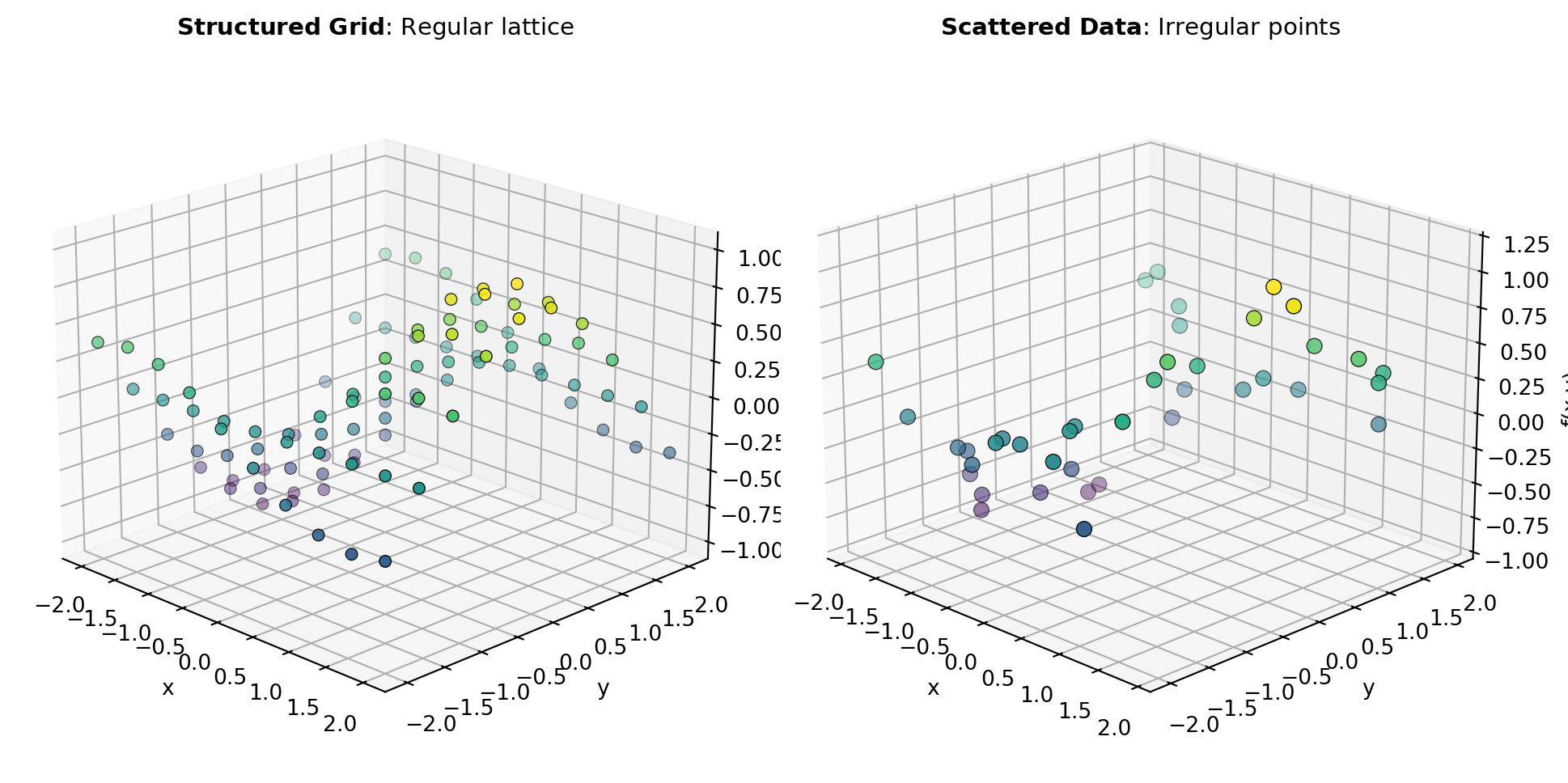
Data Arrangement: Multivariate interpolation problems fall into two categories based on data layout. Structured/gridded data has measurements at regular lattice points, forming a tensor product structure. Unstructured/scattered data arrives at arbitrary locations without regular spacing. Figure 1 illustrates how different interpolation strategies address these configurations.
Grid-Based Methods: When data lies on a regular grid, specialized methods exploit the structure for efficiency. The GRID_INTERP and INTERPN tools handle multidimensional grids by performing sequential 1-D interpolations along each axis, reducing computational complexity. These methods excel for structured data because they leverage tensor product structure and support fast indexing.
Scattered Data Methods: Unstructured data points require different approaches. The GRIDDATA tool reconstructs functions from scattered observations using triangulation-based methods, while the LINEAR_ND_INTERP tool performs piecewise linear interpolation on simplicial tessellations. For highly irregular geometries, the NEAREST_ND_INTERP tool provides fast nearest-neighbor approximation, trading smoothness for computational speed.
Radial Basis Functions: For maximum flexibility and smoothness across arbitrary point distributions, the RBF_INTERPOLATOR tool constructs global interpolants by centering basis functions at data points. Radial basis function methods provide smooth, infinitely differentiable results suitable for accurate reconstruction but require solving dense linear systems, which scales poorly to very large datasets.
Tools
| Tool | Description |
|---|---|
| GRID_INTERP | Interpolator on a regular grid in 2D. |
| GRIDDATA | Interpolate unstructured D-D data. |
| INTERPN | Multidimensional interpolation on regular grids (2D). |
| LINEAR_ND_INTERP | Piecewise linear interpolator in N > 1 dimensions. |
| NEAREST_ND_INTERP | Nearest neighbor interpolation in N > 1 dimensions. |
| RBF_INTERPOLATOR | Radial basis function interpolation in N dimensions. |