Splines
Overview
Spline interpolation is a powerful mathematical technique for constructing smooth curves through a set of data points. Unlike polynomial interpolation, which uses a single high-degree polynomial that can exhibit wild oscillations (Runge’s phenomenon), spline methods piece together multiple low-degree polynomials to create a function that is both smooth and well-behaved. The term “spline” originated from the flexible wooden or metal strips that draftsmen used to draw smooth curves through control points.
Spline interpolation emerged as a practical solution to the limitations of classical polynomial fitting. When a single polynomial of high degree is fit to many data points, the result often oscillates wildly between the data points, particularly near the edges. This oscillatory behavior is known as Runge’s phenomenon and makes high-degree polynomial interpolation unsuitable for most real-world applications. Splines solve this problem by using piecewise polynomials—rather than fitting one polynomial to all the data, multiple low-degree polynomials are connected smoothly at the data points (called knots). This approach provides excellent accuracy while maintaining computational efficiency.
B-splines (basis splines) are the foundation of modern spline interpolation. A B-spline is a piecewise polynomial function defined by control points and a knot vector. The degree of the polynomial and the spacing of knots determine the shape and smoothness of the resulting curve. Cubic splines are by far the most common choice in practice—they use degree-3 polynomials and provide an excellent balance between flexibility and computational cost, with continuous second derivatives (smoothness).
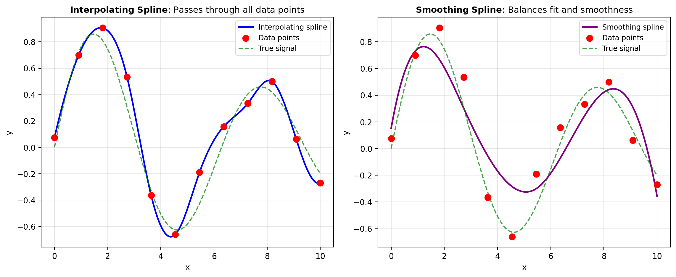
Interpolating splines pass exactly through all the specified data points, making them ideal when your data points are known to be accurate and reliable. These are implemented through the MAKE_INTERP_SPLINE and INTERP_UV_SPLINE functions.
Smoothing splines differ fundamentally from interpolating splines—rather than passing through every data point, they approximate the data while minimizing roughness. Smoothing is essential when your data contains measurement noise or measurement error. The smoothing parameter controls the trade-off between fitting the data closely and maintaining a smooth curve. Two primary implementations are available: SMOOTH_SPLINE for classical smoothing splines and UNIVARIATE_SPLINE for more flexible univariate spline fitting.
Least-squares fitting splines (MAKE_LSQ_SPLINE) represent another important variant. These splines don’t necessarily pass through any specific data points but instead minimize the sum of squared errors across many data points. This approach is particularly valuable when you have large numbers of data points and want to reduce computational complexity, or when you want to enforce specific knot locations.
Spline interpolation and smoothing are implemented through the SciPy library, specifically the scipy.interpolate module. This module provides highly optimized implementations of various spline techniques, including B-spline representation, evaluation, and fitting. The implementations use efficient algorithms that scale well with large datasets and support evaluation at arbitrary points along the spline. Beyond SciPy, NumPy provides the underlying array structures and numerical operations.
Splines are fundamental in computer graphics (defining smooth curves and surfaces for animation and visualization), data science (smoothing noisy measurements and performing nonparametric regression), engineering (modeling aerodynamic surfaces and mechanical components), and statistics (fitting flexible nonparametric models to data). The power of splines lies in their ability to balance two competing goals: fidelity to the data and smoothness of the resulting function.
Figure 1 illustrates how different spline approaches handle a dataset with varying noise levels. The comparison shows how interpolating splines pass through all points, smoothing splines reduce noise while capturing the underlying trend, and how the choice of method affects the final curve.
Tools
| Tool | Description |
|---|---|
| INTERP_UV_SPLINE | 1-D interpolating spline for data. |
| MAKE_INTERP_SPLINE | Compute interpolating B-spline and evaluate at new points. |
| MAKE_LSQ_SPLINE | Compute LSQ-based fitting B-spline. |
| SMOOTH_SPLINE | Smoothing cubic spline. |
| UNIVARIATE_SPLINE | 1-D smoothing spline fit to data. |