Least Squares
Overview
Least squares is a mathematical optimization technique for finding the parameters of a model that best fit a set of observations by minimizing the sum of the squared differences (residuals) between observed and predicted values. Originally developed by Carl Friedrich Gauss and Adrien-Marie Legendre in the early 19th century, least squares has become the cornerstone of regression analysis, parameter estimation, and curve fitting across virtually every scientific and engineering discipline.
The fundamental principle is elegantly simple: given a model f(x; \theta) with parameters \theta and observed data pairs (x_i, y_i), find the parameter values that minimize the residual sum of squares (RSS):
S(\theta) = \sum_{i=1}^{n} \left(y_i - f(x_i; \theta)\right)^2
When the model is linear in its parameters, the solution is analytical and exact. When the model is nonlinear, iterative numerical optimization algorithms are required. The resulting parameter estimates have well-understood statistical properties, particularly when errors are normally distributed: the least-squares estimator is unbiased, has minimum variance among all linear unbiased estimators (Gauss-Markov theorem), and provides the foundation for hypothesis testing and confidence interval construction.
Implementation: Least squares fitting is supported across multiple Python ecosystems. SciPy provides the versatile curve_fit function for general-purpose optimization. lmfit builds on SciPy with high-level models and intuitive parameter management. CasADi enables symbolic optimization with automatic differentiation for complex models. iminuit provides robust Minuit-based fitting with detailed uncertainty estimates.
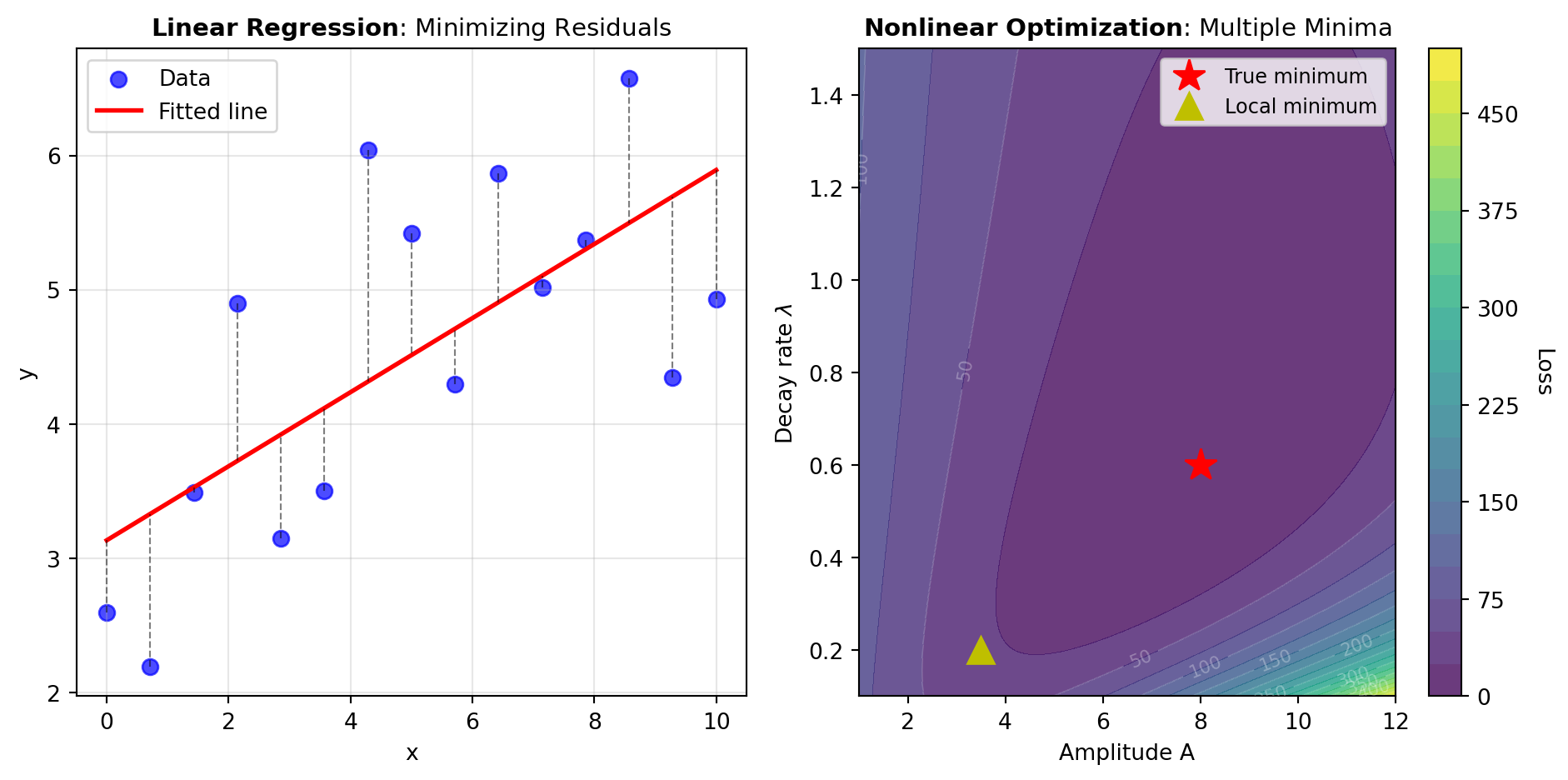
Linear vs. Nonlinear Models: Linear models—where parameters appear as weighted sums—yield closed-form solutions through normal equations or direct decomposition methods. Examples include polynomial regression, where the model is f(x) = a_0 + a_1 x + a_2 x^2 + \ldots, and multiple regression. Nonlinear models require iterative optimization: exponential decay f(x) = A e^{-\lambda x}, power laws f(x) = a x^b, or sigmoidal growth. The optimization landscape for nonlinear problems can be complex, with multiple local minima requiring careful initialization.
Model Selection and Diagnostics: Choosing an appropriate model is as important as fitting it. Information criteria like Akaike (AIC) and Bayesian (BIC) criteria balance model complexity with fit quality, penalizing overfitting. Residual analysis—examining the pattern of differences between data and predictions—reveals systematic deviations and violations of modeling assumptions. The coefficient of determination (R^2) quantifies the fraction of variance explained.
Weighted Least Squares: When observations have different measurement uncertainties or are drawn from heteroscedastic distributions (where variance changes across the domain), weighting provides better parameter estimates and more accurate uncertainty quantification. Observations with smaller uncertainties receive higher weights: S(\theta) = \sum_{i=1}^{n} w_i (y_i - f(x_i; \theta))^2, where w_i = 1/\sigma_i^2.
Optimization Tools: The tools in this category span different use cases. The CURVE_FIT tool handles straightforward function fitting with scipy. The LM_FIT tool provides a higher-level interface with built-in models and flexible composition. For symbolic models requiring automatic differentiation, CA_CURVE_FIT leverages CasADi. The MINUIT_FIT tool specializes in detailed uncertainty estimation using iminuit’s robust algorithms.
Figure 1 illustrates the core least squares concepts: how residuals are computed and minimized, and how the optimization landscape differs between linear and nonlinear problems.
Tools
| Tool | Description |
|---|---|
| CA_CURVE_FIT | Fit an arbitrary symbolic model to data using CasADi and automatic differentiation. |
| CURVE_FIT | Fit a model expression to xdata, ydata using scipy.optimize.curve_fit. |
| LM_FIT | Fit data using lmfit’s built-in models with optional model composition. |
| MINUIT_FIT | Fit an arbitrary model expression to data using iminuit least-squares minimization with uncertainty estimates. |