Optimization
Overview
Optimization is the mathematical discipline concerned with finding the “best” solution from a set of feasible alternatives. At its core, an optimization problem consists of three components: an objective function to minimize or maximize, a set of decision variables that can be adjusted, and a collection of constraints that define the feasible region. This framework is remarkably versatile and appears throughout science, engineering, economics, and business operations.
Problem Structure and Formulation
A mathematical optimization problem is typically expressed as: minimize or maximize f(x) subject to constraints g(x) \leq 0, h(x) = 0, and x \in \mathbb{R}^n. The objective function f maps decision variables to a scalar value we seek to optimize, while constraints define the feasible region—the set of acceptable solutions. Problems vary dramatically in structure: some have linear objectives and constraints, others are highly nonlinear, and still others involve discrete (integer) variables. The structure of your problem determines which algorithm is most suitable.
Application Domains
In operations research, optimization drives logistics, supply chain management, and resource allocation decisions that can involve thousands of variables and constraints. In economics and finance, portfolio optimization balances risk and return while managing constraints on capital and diversification. Engineering applications range from structural design and control systems to parameter tuning and model fitting. In machine learning, training neural networks is fundamentally an optimization problem where gradient-based methods adjust millions of parameters to minimize a loss function.
Python Implementation Libraries
The primary library for optimization in Python is SciPy, which provides robust, well-tested implementations of classical optimization algorithms. SciPy’s scipy.optimize module covers univariate and multivariate optimization, root finding, linear programming, and more. For more advanced applications involving automatic differentiation and flexible model specification, CasADi offers symbolic computation and efficient optimization with automatic Jacobian/Hessian computation. These libraries implement algorithms ranging from simple gradient descent to sophisticated metaheuristic approaches.
Optimization Categories and When to Use Them
Local Optimization finds local minima of smooth functions using gradient-based methods (derivatives). Use these when the function is differentiable and you have a good starting point near the true minimum. The MINIMIZE tool handles general multivariate problems with optional constraints, while MINIMIZE_SCALAR specializes in single-variable functions. CA_MINIMIZE leverages CasADi’s automatic differentiation for complex expressions.
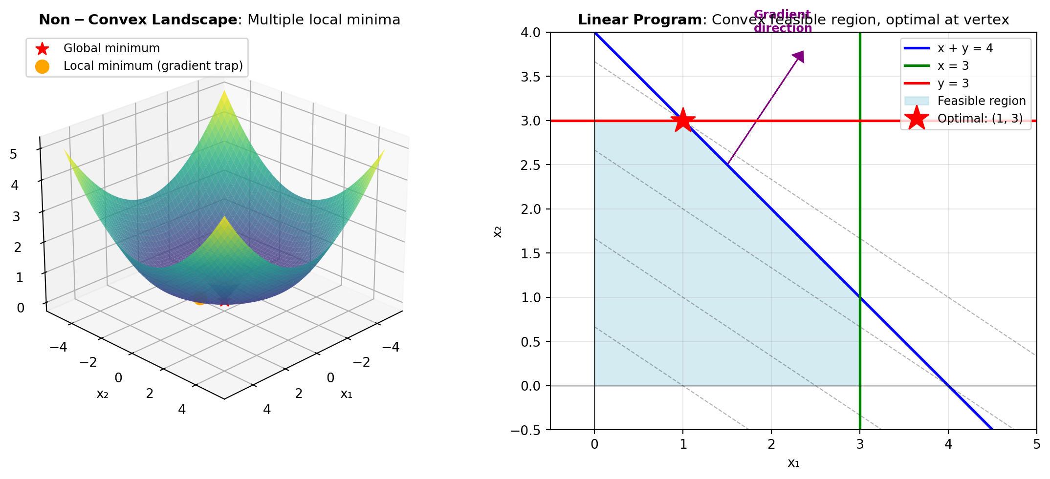
Global Optimization searches for the best solution across the entire feasible region, not just locally. This is essential when the objective function is non-convex or has multiple local minima. Methods include stochastic approaches like DIFF_EVOLUTION and DUAL_ANNEALING, which probabilistically escape local optima, exhaustive methods like BRUTE force grid search, and specialized algorithms like BASIN_HOPPING and SHGO. Use global optimization when you cannot guarantee your starting point is near the true optimum.
Linear Programming solves problems where both the objective and constraints are linear in the decision variables. These problems have efficient polynomial-time solutions. Use LINEAR_PROG for continuous linear programs and MILP when variables must be integers or mixed integer-continuous. CA_QUAD_PROG extends this to quadratic objectives, which also have efficient solvers.
Root Finding solves systems of equations f(x) = 0. While superficially different from optimization, root finding is mathematically equivalent to finding where the gradient equals zero. Use ROOT for systems of nonlinear equations, ROOT_SCALAR for single-variable equations, and CA_ROOT when automatic differentiation is beneficial. The FIXED_POINT tool finds solutions to f(x) = x, common in iterative algorithms.
Assignment Problems assign n workers to n tasks optimally. These special-structure problems have dedicated efficient solvers. Use LINEAR_ASSIGNMENT for classical assignment problems with linear costs, and QUAD_ASSIGN when the cost depends quadratically on the assignment pattern.
Assignment Problems
| Tool | Description |
|---|---|
| LINEAR_ASSIGNMENT | Solve the linear assignment problem using scipy.optimize.linear_sum_assignment. |
| QUAD_ASSIGN | Solve a quadratic assignment problem using SciPy’s implementation. |
Global Optimization
| Tool | Description |
|---|---|
| BASIN_HOPPING | Minimize a single-variable expression with SciPy’s basinhopping algorithm. |
| BRUTE | Perform a brute-force grid search to approximate the global minimum of a function. |
| DIFF_EVOLUTION | Minimize a multivariate function using differential evolution. |
| DUAL_ANNEALING | Minimize a multivariate function using dual annealing. |
| SHGO | Find global minimum using Simplicial Homology Global Optimization. |
Linear Programming
| Tool | Description |
|---|---|
| CA_QUAD_PROG | Solve a quadratic programming problem using CasADi’s qpsol solver. |
| LINEAR_PROG | Solve a linear programming problem using SciPy’s linprog function. |
| MILP | Solve a mixed-integer linear program using scipy.optimize.milp. |
Local Optimization
| Tool | Description |
|---|---|
| CA_MINIMIZE | Minimize a multivariate function using CasADi with automatic differentiation. |
| MINIMIZE | Minimize a multivariate function using SciPy’s minimize routine. |
| MINIMIZE_SCALAR | Minimize a single-variable function using SciPy’s minimize_scalar. |
Root Finding
| Tool | Description |
|---|---|
| CA_ROOT | Solve a system of nonlinear equations using CasADi with automatic Jacobian. |
| FIXED_POINT | Find a fixed point x such that f(x) = x for a scalar function expression. |
| ROOT | Solve a square nonlinear system using SciPy’s root solver. |
| ROOT_SCALAR | Find a real root of a scalar function using SciPy’s root_scalar. |