Ode Systems
Overview
Ordinary differential equations (ODEs) form the mathematical backbone for modeling dynamic systems across virtually every scientific and engineering discipline. An ODE describes how a system’s state changes over time through relationships between functions and their derivatives. The canonical form \frac{dy}{dt} = f(t, y) expresses the rate of change of the state y as a function of time t and the current state itself. While simple in concept, ODEs can capture remarkably complex phenomena—from orbital mechanics and chemical reaction networks to population dynamics and electrical circuits. The beauty of differential equations lies in their universality: the same mathematical framework describes a predator-prey ecosystem, a heated rod cooling in air, or a spacecraft orbiting the Earth.
The Solution Challenge: Finding the function y(t) that satisfies a differential equation is far from straightforward. Analytical solutions exist for only a narrow class of special cases—linear ODEs with constant coefficients, separable equations, and a few other carefully structured families. The vast majority of real-world systems exhibit nonlinear dynamics that resist closed-form solutions. This is where numerical methods become essential. Rather than seeking an exact symbolic answer, these algorithms discretize time into small steps and iteratively compute approximate values of the solution at each step, building up an accurate trajectory through state space.
Implementation Approaches: The tools in this category leverage NumPy and SciPy’s integrate module, which implements production-grade numerical ODE solvers including explicit Runge-Kutta methods, implicit methods for stiff systems, and advanced adaptive step-size control. These bring sophisticated algorithms and automatic error handling directly into Excel.
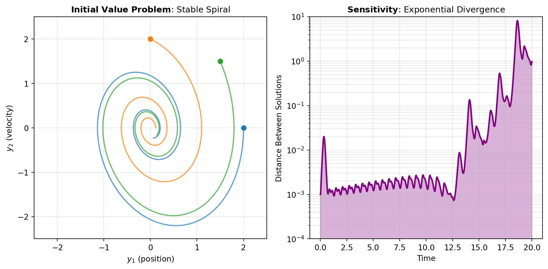
Initial Value Problems (IVPs): The most common scenario involves specifying the state at an initial time and integrating forward to find the state at future times. Figure 1(A) illustrates this concept: given y(t_0) = y_0 and the differential equation, we trace the trajectory through time. The SOLVE_IVP tool handles systems of first-order ODEs of the form \frac{dy}{dt} = Ay where A is a system matrix. This class of linear systems arises frequently in control theory, mechanical vibrations, coupled electrical circuits, and chemical kinetics. The solver automatically selects appropriate numerical methods (explicit for non-stiff systems, implicit for stiff systems) and ensures the error remains below user-specified tolerances throughout integration.
Boundary Value Problems (BVPs): A complementary class of problems specifies conditions at both endpoints rather than just an initial condition. For instance, finding the shape of a hanging cable requires knowing both the position at the left support and the position at the right support—but not the vertical velocities at those points. Boundary value problems are intrinsically harder than initial value problems because the solution information is distributed across the domain, preventing straightforward forward integration. The SOLVE_BVP tool handles second-order systems with boundary conditions at both endpoints using a finite-difference shooting method that iteratively adjusts initial conditions until the final boundary conditions are satisfied.
Numerical Stability Considerations: Real-world systems often involve widely different timescales—fast chemical reactions coupled with slow thermal diffusion, for example. These stiff systems require special care: standard explicit methods become prohibitively slow because they must use tiny time steps to maintain stability. Modern solvers like those in SciPy automatically detect stiffness and switch to implicit methods that handle rapid transients accurately while taking larger steps through slower dynamics.
Figure 1 also shows how two different systems with identical initial conditions can diverge dramatically due to nonlinear feedback, highlighting why numerical accuracy is critical for trustworthy predictions in chaotic or sensitive systems.
Tools
| Tool | Description |
|---|---|
| SOLVE_BVP | Solve a boundary value problem for a second-order system of ODEs. |
| SOLVE_IVP | Solve an initial value problem for a system of ODEs of the form dy/dt = A @ y. |