Approximation
Overview
Approximation theory addresses a fundamental problem in numerical analysis and applied mathematics: how to represent a complex or unknown function using simpler, more tractable mathematical forms. While interpolation constructs functions that pass exactly through a given set of data points, approximation encompasses a broader class of techniques that includes polynomial approximation, rational function approximation, and least-squares fitting. The goal is to find a manageable mathematical expression that captures the essential behavior of the target function, balancing accuracy with computational efficiency.
In scientific computing, approximation methods are essential for evaluating special functions, solving differential equations, accelerating numerical algorithms, and compressing data representations. These techniques appear throughout numerical analysis, control systems engineering, signal processing, and computational physics. By replacing expensive function evaluations with simpler polynomial or rational expressions, approximation methods enable faster simulations and analytical insights into system behavior. Function evaluation cost reduction is a key benefit: evaluating a transcendental function like \sin(x) or e^x on a processor is expensive; evaluating a simple polynomial is cheap.
Implementation: The tools in this category leverage SciPy and NumPy for robust numerical computation of approximating functions. SciPy’s interpolate module provides specialized algorithms optimized for stability and accuracy across diverse domains.
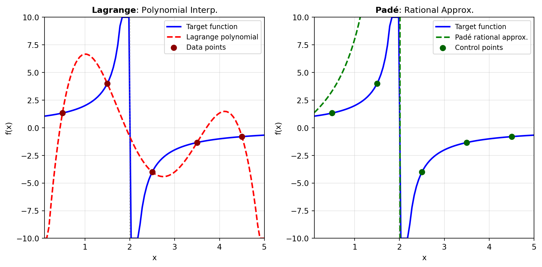
Polynomial Approximation: The LAGRANGE_INTERP tool constructs the Lagrange interpolating polynomial through a given set of data points. This fundamental technique in numerical analysis generates the unique polynomial of lowest degree passing through specified points. Lagrange polynomials excel for small numbers of data points and serve as the foundation for many numerical methods including integration and differentiation. The method works by constructing basis polynomials, each equal to one at its corresponding data point and zero at all others. However, Lagrange interpolation exhibits important numerical challenges: the direct formulation becomes unstable for more than approximately 20 points, and equally-spaced interpolation nodes can trigger Runge’s phenomenon—oscillatory artifacts near the boundaries of the interpolation interval.
Rational Approximation: The PADE tool computes Padé rational approximants, expressing functions as the ratio of two polynomials. Named after Henri Padé, this technique often outperforms polynomial approximation, particularly near singularities or where Taylor series converge slowly or diverge. A Padé approximant of order [m/n] is a rational function where numerator and denominator polynomials have degrees m and n, with coefficients chosen so the Taylor series expansion matches the original function to order m + n. This approach excels at representing functions with poles (like 1/(1-x)), branch cuts, and transcendental functions (exponentials, logarithms, trigonometric functions). A classic example is the [2/2] Padé approximant of e^x, which provides excellent accuracy across a wide range with only a simple rational expression, vastly outperforming a quadratic Taylor polynomial.
Choosing Between Approximation Methods: Use polynomial approximation when you need simplicity, have few interpolation points, or require exact values at specific locations. Choose rational approximation when dealing with functions exhibiting poles, when you need better accuracy with fewer terms, or when approximating functions with singularities. Figure 1 illustrates how these methods complement each other in capturing function behavior with different characteristics.
Tools
| Tool | Description |
|---|---|
| LAGRANGE_INTERP | Compute the Lagrange interpolating polynomial through a set of points. |
| PADE | Compute Pade rational approximation to a polynomial. |