Math

Overview

Mathematical computation forms the backbone of quantitative analysis in science, engineering, finance, and data science. This comprehensive library of mathematical functions extends Excel’s capabilities far beyond native formulas, providing access to sophisticated numerical methods implemented in SciPy, NumPy, CasADi, and specialized Python libraries.

Modern mathematical computing requires far more than basic arithmetic—it demands robust algorithms for solving differential equations, fitting complex models to data, optimizing multivariate functions, and performing matrix operations with numerical stability. These functions bridge the gap between Excel’s spreadsheet interface and the power of production-grade scientific computing libraries, enabling researchers and engineers to tackle challenging mathematical problems directly from within a familiar spreadsheet environment.

Calculus and Differential Equations form the foundation for modeling dynamic systems. Whether computing derivatives of multivariable functions through differentiation, evaluating integrals numerically, or solving systems of ordinary differential equations, these tools enable accurate analysis of continuous change. Applications range from sensitivity analysis in optimization to pharmacokinetic modeling in drug development and epidemic modeling in public health.

Curve Fitting and Data Approximation allow you to discover the relationships hidden within data. Using least-squares regression, you can fit symbolic models or pre-defined curves to experimental measurements. This is essential across fields: chemists use adsorption and binding models to understand molecular interactions; biologists apply dose-response and enzyme kinetics models; engineers work with rheological and spectroscopic models. Advanced methods like CasADi-based fitting provide automatic differentiation for complex symbolic expressions, while spline-based interpolation reconstructs smooth curves from scattered or structured data.

Interpolation and Approximation bridge discrete data points with smooth continuous functions. Methods range from simple univariate splines and polynomial interpolation to sophisticated multidimensional approaches like radial basis functions. These are invaluable when you need to evaluate functions at arbitrary points, smooth noisy measurements, or reconstruct surfaces from scattered measurements.

Linear Algebra provides the computational foundation for modern numerical analysis. From matrix decompositions (QR, SVD, Cholesky) to solving linear systems and pseudoinverse computations, these operations underpin virtually every scientific computation. They are essential for solving overdetermined and underdetermined systems, analyzing system stability through eigenvalue problems, and transforming data for machine learning applications.

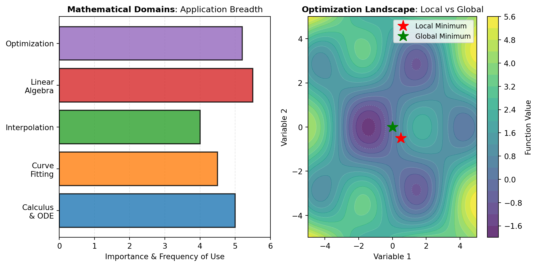
Optimization addresses the central computational challenge: finding the best solution within constraints. Assignment problems like the Hungarian algorithm match resources optimally. Local methods converge rapidly near a solution, suitable when good starting points are available. Global methods like differential evolution and dual annealing explore broader solution spaces to escape local minima. Linear and quadratic programming handle structured problems efficiently, while root-finding tools solve systems of nonlinear equations that arise throughout engineering and science. The reference figure illustrates these key mathematical domains and their interconnections.

Figure 1: Mathematical Computing Landscape: (A) Core mathematical domains and their primary applications. (B) Optimization landscape showing local minima and global structure.

Calculus

Differentiation

Tool	Description
HESSIAN	Compute the Hessian matrix (second derivatives) of a scalar function using CasADi symbolic differentiation.
JACOBIAN	Calculate the Jacobian matrix of mathematical expressions with respect to specified variables.
SENSITIVITY	Compute the sensitivity of a scalar model with respect to its parameters using CasADi.

Integration

Tool	Description
DBLQUAD	Compute the double integral of a function over a two-dimensional region.
QUAD	Numerically integrate a function defined by a table of x, y values over [a, b] using adaptive quadrature.
TRAPEZOID	Integrate sampled data using the composite trapezoidal rule.

Ode Models

Tool	Description
BRUSSELATOR	Numerically solves the Brusselator system of ordinary differential equations for autocatalytic chemical reactions.
COMPARTMENTAL_PK	Numerically solves the basic one-compartment pharmacokinetics ODE using scipy.integrate.solve_ivp.
FITZHUGH_NAGUMO	Numerically solves the FitzHugh-Nagumo system of ordinary differential equations for neuron action potentials using scipy.integrate.solve_ivp.
HODGKIN_HUXLEY	Numerically solves the Hodgkin-Huxley system of ordinary differential equations for neuron action potentials.
LORENZ	Numerically solves the Lorenz system of ordinary differential equations for chaotic dynamics.
LOTKA_VOLTERRA	Numerically solves the Lotka-Volterra predator-prey system of ordinary differential equations.
MICHAELIS_MENTEN	Numerically solves the Michaelis-Menten system of ordinary differential equations for enzyme kinetics using scipy.integrate.solve_ivp.
SEIR	Numerically solves the SEIR system of ordinary differential equations for infectious disease modeling using scipy.integrate.solve_ivp.
SIR	Solves the SIR system of ordinary differential equations for infection dynamics using scipy.integrate.solve_ivp (see scipy.integrate.solve_ivp).
VAN_DER_POL	Numerically solves the Van der Pol oscillator system of ordinary differential equations.

Ode Systems

Tool	Description
SOLVE_BVP	Solve a boundary value problem for a second-order system of ODEs.
SOLVE_IVP	Solve an initial value problem for a system of ODEs of the form dy/dt = A @ y.

Curve Fitting

Least Squares

Tool	Description
CA_CURVE_FIT	Fit an arbitrary symbolic model to data using CasADi and automatic differentiation.
CURVE_FIT	Fit a model expression to xdata, ydata using scipy.optimize.curve_fit.
LM_FIT	Fit data using lmfit’s built-in models with optional model composition.
MINUIT_FIT	Fit an arbitrary model expression to data using iminuit least-squares minimization with uncertainty estimates.

Models

Tool	Description
ADSORPTION	Fits adsorption models to data using scipy.optimize.curve_fit.
AGRICULTURE	Fits agriculture models to data using scipy.optimize.curve_fit.
BINDING_MODEL	Fits binding_model models to data using scipy.optimize.curve_fit.
CHROMA_PEAKS	Fits chroma_peaks models to data using scipy.optimize.curve_fit.
DOSE_RESPONSE	Fits dose_response models to data using scipy.optimize.curve_fit.
ELECTRO_ION	Fits electro_ion models to data using scipy.optimize.curve_fit.
ENZYME_BASIC	Fits enzyme_basic models to data using scipy.optimize.curve_fit.
ENZYME_INHIBIT	Fits enzyme_inhibit models to data using scipy.optimize.curve_fit.
EXP_ADVANCED	Fits exp_advanced models to data using scipy.optimize.curve_fit.
EXP_DECAY	Fits exp_decay models to data using scipy.optimize.curve_fit.
EXP_GROWTH	Fits exponential growth models to data using scipy.optimize.curve_fit.
GROWTH_POWER	Fits growth_power models to data using scipy.optimize.curve_fit.
GROWTH_SIGMOID	Fits growth_sigmoid models to data using scipy.optimize.curve_fit.
MISC_PIECEWISE	Fits misc_piecewise models to data using scipy.optimize.curve_fit.
PEAK_ASYM	Fits peak_asym models to data using scipy.optimize.curve_fit.
POLY_BASIC	Fits poly_basic models to data using scipy.optimize.curve_fit.
RHEOLOGY	Fits rheology models to data using scipy.optimize.curve_fit.
SPECTRO_PEAKS	Fits spectro_peaks models to data using scipy.optimize.curve_fit.
STAT_DISTRIB	Fits stat_distrib models to data using scipy.optimize.curve_fit.
STAT_PARETO	Fits stat_pareto models to data using scipy.optimize.curve_fit.
WAVEFORM	Fits waveform models to data using scipy.optimize.curve_fit.

Geometry

Gis

Tool	Description
SHAPELY_AREA	Calculate the area of a geometry.
SHAPELY_BUFFER	Returns a representation of all points within a given distance of the this geometric object.
SHAPELY_CONTAINS	Returns True if the first geometry contains the second.
SHAPELY_CONVEX_HULL	Returns the smallest convex polygon that contains all the points in the object.
SHAPELY_DISTANCE	Calculate the minimum distance between two geometries.
SHAPELY_INTERSECT	Returns a representation of the intersection of this object with another geometric object.
SHAPELY_LINESTRING	Create a geometric line string from a list of points.
SHAPELY_PLOT	Plot geometries and return an image.
SHAPELY_POINT	Create a geometric point.
SHAPELY_POLYGON	Create a geometric polygon from a shell of points and optional holes.
SHAPELY_SIMPLIFY	Returns a simplified representation of the geometric object.
SHAPELY_UNION_ALL	Returns the union of all geometries in the input list.

Triangle Solvers

Tool	Description
TRI_AAAS	Solve a triangle from three angles and one side for scale.
TRI_SAS	Solve a triangle from two sides and their included angle.
TRI_SOLVE	Solve a triangle from any valid combination of three known side/angle values.
TRI_SSA	Solve a triangle from two sides and a non-included angle using SSA branch selection.
TRI_SSS	Solve a triangle from three known side lengths.

Trig Identities

Tool	Description
TRIG_EXPAND	Expand trigonometric compound-angle expressions into component terms.
TRIG_FU	Simplify trigonometric expressions using the Fu transformation pipeline.
TRIG_TR1	Rewrite secant and cosecant into reciprocal cosine and sine forms.
TRIG_TR10	Expand sine and cosine of summed angles into separated component terms.
TRIG_TR2	Rewrite tangent and cotangent into sine-cosine ratio forms.
TRIG_TR3	Normalize trig signs and induced odd/even identity forms.
TRIG_TR4	Evaluate exact trigonometric values at standard special angles.
TRIG_TR5	Replace even powers of sine using a cosine-based identity.
TRIG_TR6	Replace even powers of cosine using a sine-based identity.
TRIG_TR7	Apply power-reduction to cosine-squared terms.
TRIG_TR8	Convert products of sine and cosine terms into sum or difference forms.
TRIG_TR9	Convert sums of sine or cosine terms into product forms.
TRIG_TRIGSIMP	Simplify a trigonometric expression using identity transformations.

Graph Theory

Centrality

Tool	Description
BETWEENNESS_CENT	Calculate the shortest-path betweenness centrality for nodes.
CLOSENESS_CENT	Calculate the closeness centrality for nodes.
DEGREE_CENTRALITY	Calculate the degree centrality for nodes in a graph.
EIGENVECTOR_CENT	Calculate the eigenvector centrality for nodes.
PAGERANK	Calculate the PageRank of the nodes in the graph.

Network Flow

Tool	Description
MAX_FLOW_VALUE	Calculate the maximum flow value between a source and sink.
MIN_COST_FLOW_COST	Find the minimum cost to satisfy all demands in a network.
MIN_CUT_VALUE	Calculate the capacity of the minimum (source, sink) cut.

Shortest Path

Tool	Description
MIN_SPANNING_TREE	Find the minimum spanning tree (MST) of an undirected graph.
SHORTEST_PATH	Find the shortest path and its length between two nodes in a network.

Interpolation

Approximation

Tool	Description
LAGRANGE_INTERP	Compute the Lagrange interpolating polynomial through a set of points.
PADE	Compute Pade rational approximation to a polynomial.

Multivariate

Tool	Description
GRID_INTERP	Interpolator on a regular grid in 2D.
GRIDDATA	Interpolate unstructured D-D data.
INTERPN	Multidimensional interpolation on regular grids (2D).
LINEAR_ND_INTERP	Piecewise linear interpolator in N > 1 dimensions.
NEAREST_ND_INTERP	Nearest neighbor interpolation in N > 1 dimensions.
RBF_INTERPOLATOR	Radial basis function interpolation in N dimensions.

Splines

Tool	Description
INTERP_UV_SPLINE	1-D interpolating spline for data.
MAKE_INTERP_SPLINE	Compute interpolating B-spline and evaluate at new points.
MAKE_LSQ_SPLINE	Compute LSQ-based fitting B-spline.
SMOOTH_SPLINE	Smoothing cubic spline.
UNIVARIATE_SPLINE	1-D smoothing spline fit to data.

Univariate

Tool	Description
AKIMA_INTERP	Akima 1D interpolation.
BARYCENTRIC_INTERP	Interpolating polynomial for a set of points using barycentric interpolation.
CUBIC_SPLINE	Cubic spline data interpolator.
HERMITE_SPLINE	Piecewise-cubic interpolator matching values and first derivatives.
INTERP1D	Interpolate a 1-D function.
KROGH_INTERPOLATE	Krogh polynomial interpolation.
PCHIP_INTERPOLATE	PCHIP 1-D monotonic cubic interpolation.

Linear Algebra

Decompositions

Tool	Description
CHOLESKY	Compute the Cholesky decomposition of a real, symmetric positive-definite matrix.
HESSENBERG	Compute Hessenberg form of a matrix.
LDL	Compute the LDLt or Bunch-Kaufman factorization of a symmetric matrix.
LU	Compute LU decomposition of a matrix with partial pivoting.
POLAR	Compute the polar decomposition of a matrix.
QR	Compute the QR decomposition of a matrix and return either Q or R.
SCHUR	Compute Schur decomposition of a matrix.
SVD	Compute the Singular Value Decomposition (SVD) of a matrix using scipy.linalg.svd.

Eigenvalues

Tool	Description
EIG	Compute eigenvalues and eigenvectors of a general square matrix.
EIGH	Solve eigenvalue problem for a real symmetric or complex Hermitian matrix.
EIGVALS	Compute eigenvalues of a general square matrix.
EIGVALSH	Compute eigenvalues of a real symmetric or complex Hermitian matrix.

Equations

Tool	Description
LSQ_LINEAR	Solve a bounded linear least-squares problem.
LSTSQ	Compute the least-squares solution to Ax = B using scipy.linalg.lstsq.
SOLVE	Solve a linear matrix equation, or system of linear scalar equations.
SOLVE_BANDED	Solve the equation Ax = b for x, assuming A is a banded matrix.
SOLVE_TOEPLITZ	Solve a Toeplitz system using Levinson Recursion.
SOLVE_TRIANGULAR	Solve the equation Ax = b for x, assuming A is a triangular matrix.

Matrix Functions

Tool	Description
COSM	Compute the matrix cosine.
EXPM	Compute the matrix exponential of a square matrix using scipy.linalg.expm
FRAC_MAT_POW	Compute the fractional power of a square matrix.
LOGM	Compute matrix logarithm.
SINM	Compute the matrix sine.
SQRTM	Compute the matrix square root.

Matrix Operations

Tool	Description
DET	Compute the determinant of a square matrix.
INV	Compute the inverse of a square matrix.
KHATRI_RAO	Compute the Khatri-Rao product of two matrices.
KRON	Compute the Kronecker product of two matrices.
MATRIX_NORM	Compute matrix or vector norm.
PINV	Compute the Moore-Penrose pseudoinverse of a matrix using singular value decomposition (SVD).

Special Matrices

Tool	Description
CIRCULANT	Construct a circulant matrix.
HADAMARD	Construct a Hadamard matrix.
HANKEL	Construct a Hankel matrix.
HILBERT	Construct a Hilbert matrix.
PASCAL	Construct a Pascal matrix.
TOEPLITZ	Construct a Toeplitz matrix.

Number Theory

Gcd Lcm Divisors

Tool	Description
DIVCOUNT	Count divisors of an integer with optional modulus filtering.
DIVISORS	List divisors of an integer with optional proper divisor mode.
GCD	Compute the greatest common divisor of one or more integers.
ISQRT	Compute the integer square root of a nonnegative integer.
LCM	Compute the least common multiple of one or more integers.
PPY_PHI	Compute Euler’s totient function using the primePy implementation.
PROPDIVCNT	Count proper divisors of an integer with optional modulus filtering.
PROPDIVS	List proper divisors of an integer.
REDUCEDTOT	Compute Carmichael’s reduced totient function for an integer.
TOTIENT	Compute Euler’s totient function for an integer.

Modular Arithmetic

Tool	Description
DLOG	Solve discrete logarithms in modular arithmetic.
ISPRIMROOT	Check whether a value is a primitive root modulo n.
ISQUADRES	Check whether a value is a quadratic residue modulo p.
JACOBI	Compute the Jacobi symbol for two integers.
LEGENDRE	Compute the Legendre symbol modulo an odd prime.
NORDER	Find the multiplicative order of an integer modulo n.
NTHROOTMOD	Solve nth-power congruences modulo an integer.
PRIMROOT	Find a primitive root modulo n when one exists.
QUADCONG	Solve quadratic congruences modulo n.
QUADRES	List all quadratic residues modulo p.
SQRTMOD	Solve quadratic congruences of the form x squared congruent to a.

Prime Numbers

Tool	Description
FACTORINT	Compute the prime factorization of an integer with multiplicities.
ISPRIME	Determine whether an integer is prime.
NEXTPRIME	Return the ith prime number greater than a given integer.
PPY_PRIMEBETWEEN	List prime numbers between two bounds using primePy.
PPY_PRIMECHECK	Check primality using the primePy implementation.
PPY_PRIMEUPTO	List all prime numbers up to a maximum value using primePy.
PREVPRIME	Return the largest prime smaller than a given integer.
PRIME	Return the nth prime number.
PRIMEFACTORS	Return distinct prime factors of an integer.
PRIMEPI	Count the number of primes less than or equal to an integer.
PRIMERANGE	Generate all prime numbers in a specified interval.
RANDPRIME	Sample a prime number from a half-open integer interval.

Optimization

Assignment Problems

Tool	Description
LINEAR_ASSIGNMENT	Solve the linear assignment problem using scipy.optimize.linear_sum_assignment.
QUAD_ASSIGN	Solve a quadratic assignment problem using SciPy’s implementation.

Global Optimization

Tool	Description
BASIN_HOPPING	Minimize a single-variable expression with SciPy’s basinhopping algorithm.
BRUTE	Perform a brute-force grid search to approximate the global minimum of a function.
DIFF_EVOLUTION	Minimize a multivariate function using differential evolution.
DUAL_ANNEALING	Minimize a multivariate function using dual annealing.
SHGO	Find global minimum using Simplicial Homology Global Optimization.

Linear Programming

Tool	Description
CA_QUAD_PROG	Solve a quadratic programming problem using CasADi’s qpsol solver.
LINEAR_PROG	Solve a linear programming problem using SciPy’s linprog function.
MILP	Solve a mixed-integer linear program using scipy.optimize.milp.

Local Optimization

Tool	Description
CA_MINIMIZE	Minimize a multivariate function using CasADi with automatic differentiation.
MINIMIZE	Minimize a multivariate function using SciPy’s minimize routine.
MINIMIZE_SCALAR	Minimize a single-variable function using SciPy’s minimize_scalar.

Root Finding

Tool	Description
CA_ROOT	Solve a system of nonlinear equations using CasADi with automatic Jacobian.
FIXED_POINT	Find a fixed point x such that f(x) = x for a scalar function expression.
ROOT	Solve a square nonlinear system using SciPy’s root solver.
ROOT_SCALAR	Find a real root of a scalar function using SciPy’s root_scalar.

Special Functions

Bessel Functions

Tool	Description
BESSEL_HANKEL1	Compute the cylindrical Hankel function of the first kind and return real and imaginary parts.
BESSEL_HANKEL2	Compute the cylindrical Hankel function of the second kind and return real and imaginary parts.
BESSEL_IV	Compute the modified cylindrical Bessel function of the first kind for real order.
BESSEL_JN_ZEROS	Compute the first positive zeros of the integer-order Bessel function of the first kind.
BESSEL_JV	Compute the cylindrical Bessel function of the first kind for real order.
BESSEL_KV	Compute the modified cylindrical Bessel function of the second kind for real order.
BESSEL_YN_ZEROS	Compute the first positive zeros of the integer-order Bessel function of the second kind.
BESSEL_YV	Compute the cylindrical Bessel function of the second kind for real order.
SPHERICAL_IN	Compute the modified spherical Bessel function of the first kind or its derivative.
SPHERICAL_JN	Compute the spherical Bessel function of the first kind or its derivative.
SPHERICAL_KN	Compute the modified spherical Bessel function of the second kind or its derivative.
SPHERICAL_YN	Compute the spherical Bessel function of the second kind or its derivative.

Elliptic Integrals

Tool	Description
ELLIPE	Compute the complete elliptic integral of the second kind.
ELLIPEINC	Compute the incomplete elliptic integral of the second kind.
ELLIPJ	Compute Jacobi elliptic functions sn, cn, dn and amplitude for scalar input.
ELLIPK	Compute the complete elliptic integral of the first kind.
ELLIPKINC	Compute the incomplete elliptic integral of the first kind.
ELLIPKM1	Compute the complete elliptic integral of the first kind near m equals one.
ELLIPRC	Compute Carlson’s degenerate symmetric elliptic integral RC.
ELLIPRD	Compute Carlson’s symmetric elliptic integral RD.
ELLIPRF	Compute Carlson’s completely symmetric elliptic integral RF.
ELLIPRG	Compute Carlson’s completely symmetric elliptic integral RG.
ELLIPRJ	Compute Carlson’s symmetric elliptic integral RJ.

Error And Fresnel

Tool	Description
DAWSN	Evaluate Dawson’s integral for a real input.
ERF	Evaluate the Gauss error function for a real input.
ERFC	Evaluate the complementary error function for a real input.
ERFCINV	Compute the inverse complementary error function on its real domain.
ERFCX	Evaluate the exponentially scaled complementary error function.
ERFI	Evaluate the imaginary error function for a real input.
ERFINV	Compute the inverse error function on its real domain.
FRESNEL	Compute Fresnel sine and cosine integrals for a real input.
WOFZ	Compute the Faddeeva function and return real and imaginary parts.

Gamma Beta Functions

Tool	Description
BETAINC	Compute the regularized incomplete beta function.
BETAINCINV	Invert the regularized incomplete beta function with respect to x.
BETALN	Compute the natural logarithm of the absolute beta function.
DIGAMMA	Compute the digamma function for a real input.
EULER_BETA	Evaluate the Euler beta function for two real parameters.
GAMMA	Evaluate the gamma function for a real input.
GAMMAINC	Compute the regularized lower incomplete gamma function.
GAMMAINCC	Compute the regularized upper incomplete gamma function.
GAMMAINCCINV	Invert the regularized upper incomplete gamma function.
GAMMAINCINV	Invert the regularized lower incomplete gamma function.
GAMMALN	Compute the natural logarithm of the absolute gamma function.
POCH	Evaluate the rising factorial using the Pochhammer symbol.
POLYGAMMA	Compute the n-th derivative of the digamma function.
RGAMMA	Compute the reciprocal of the gamma function.