Univariate
Overview
Univariate interpolation is the process of estimating unknown values of a function between known data points. Given a set of discrete points (x_i, y_i), the goal is to construct a continuous function f(x) that passes through all the data points (f(x_i) = y_i) and can be evaluated at any intermediate value. This is fundamental in numerical analysis, data visualization, engineering simulations, and scientific computing where measured or sampled data is inherently discrete but the underlying phenomenon is continuous.
In real-world applications, data collection is often expensive, time-consuming, or physically constrained to discrete samples. Experimental measurements, sensor readings, and computational simulations all produce discrete data points. Yet the underlying physical phenomena—material properties, environmental gradients, signal characteristics—are typically continuous. Interpolation bridges this gap by reconstructing smooth functions from sparse data, enabling evaluation at any point within the domain and providing insights into the function’s overall behavior.
Implementation: The tools in this category leverage SciPy, particularly its interpolate module, which offers a wide variety of univariate interpolation methods. These implementations support both function definition and derivative computation at interpolated points, enabling seamless integration with optimization algorithms, sensitivity analysis, and scientific computing workflows.
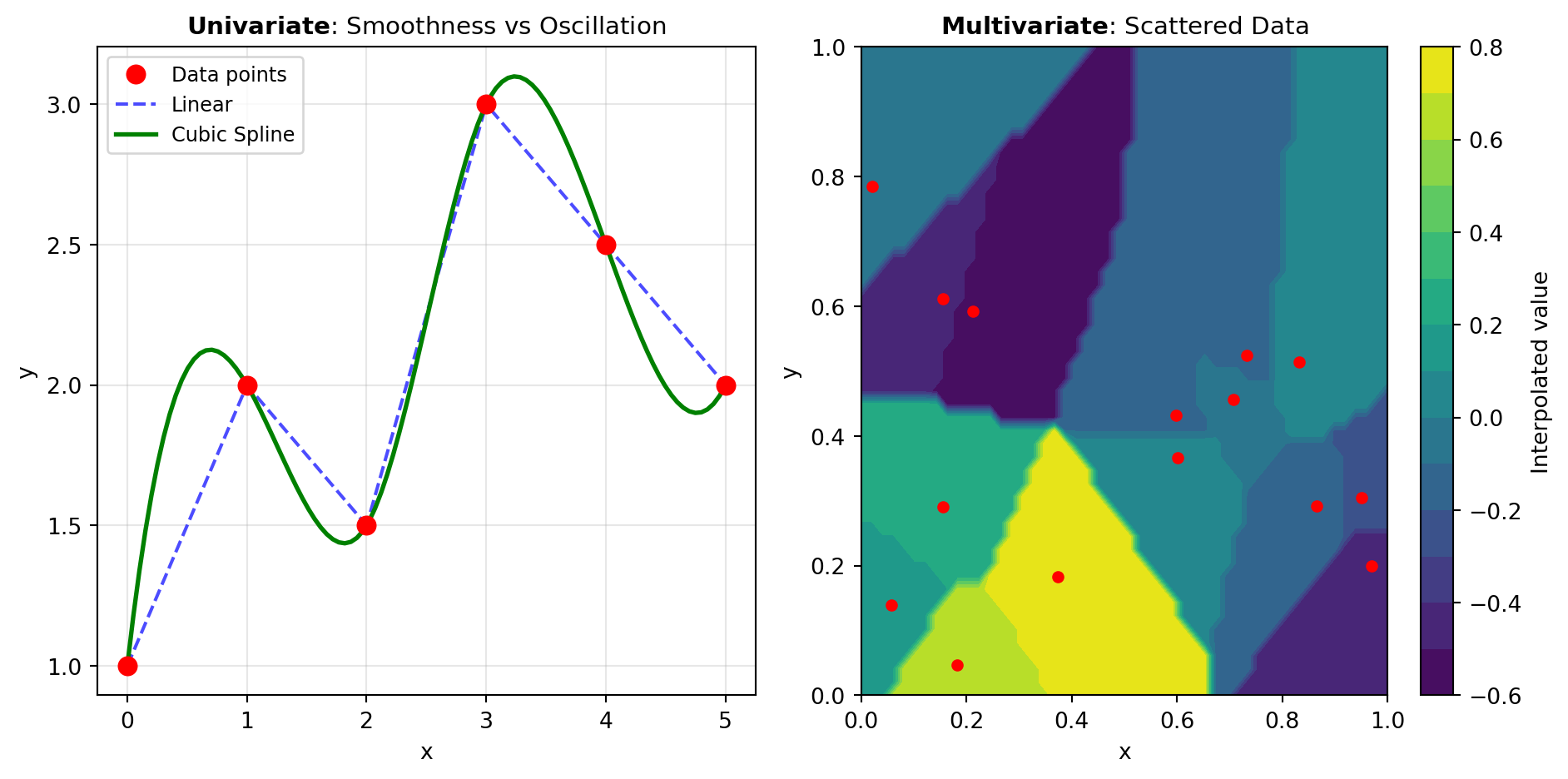
The choice of interpolation method profoundly affects the quality and behavior of the resulting function. Key considerations include the nature of the data, desired smoothness properties, computational efficiency, behavior outside the data range, and whether derivative information is available. Figure 1 illustrates two distinct approaches to univariate interpolation.
Polynomial and Global Methods: Barycentric interpolation and Krogh polynomial interpolation construct a single polynomial that passes through all data points. These methods leverage elegant mathematical properties—barycentric form is numerically stable and efficient, while Krogh interpolation naturally incorporates derivative constraints. Global methods excel when data is accurate and well-distributed, but can suffer from Runge’s phenomenon (oscillations at interval boundaries) with unevenly spaced or noisy data.
Spline-Based Methods: Rather than fitting a single polynomial, spline methods divide the data into segments and fit low-degree polynomials locally. The cubic spline is the classical choice, balancing simplicity with smoothness by ensuring continuity of position, first derivative, and second derivative. Hermite splines extend this flexibility by incorporating derivative constraints at each point, enabling shape control and matching of known slope information. These piecewise approaches avoid oscillations and handle noise more gracefully than global polynomials.
Monotonicity and Shape Preservation: Real-world data often exhibits monotonic behavior—strictly increasing or decreasing. Monotone cubic interpolation methods like PCHIP preserve this structure, preventing spurious overshooting or non-physical behavior common with unrestricted cubic splines. This is critical for data representing physical quantities with inherent directional properties, such as cumulative mass, energy dissipation, or concentration profiles.
Advanced Techniques: Akima splines provide an alternative that reduces oscillations by considering local behavior without enforcing monotonicity constraints. Linear interpolation with kind='linear' offers the simplest approach for rapid approximation, while higher-order interpolation in the general interpolation interface provides flexibility to choose the balance between accuracy and computational cost.
Understanding the trade-offs between these methods is essential. Local methods (splines) are robust and efficient, while global methods offer elegance when data quality permits. Derivative information can be incorporated where available, and shape constraints can enforce physical realism.
Tools
| Tool | Description |
|---|---|
| AKIMA_INTERP | Akima 1D interpolation. |
| BARYCENTRIC_INTERP | Interpolating polynomial for a set of points using barycentric interpolation. |
| CUBIC_SPLINE | Cubic spline data interpolator. |
| HERMITE_SPLINE | Piecewise-cubic interpolator matching values and first derivatives. |
| INTERP1D | Interpolate a 1-D function. |
| KROGH_INTERPOLATE | Krogh polynomial interpolation. |
| PCHIP_INTERPOLATE | PCHIP 1-D monotonic cubic interpolation. |